Tidymodels Regression Case study

Regression

Machine learning

Tidymodels

Published

11 January 2024

library Setup

library(tidyverse)
library(tidymodels)
library(glue)
library(lubridate)
library(patchwork)
library(scales)
library(summarytools)
library(glmnet)
library(randomForest)
library(xgboost)
library(conflicted)
library(flextable)
library(tvthemes)
slice <- dplyr::slice
eval_metrics <- metric_set(rmse, rsq)

A work by Bongani Ncube

r195334vncube@gmail.com

Introduction

This tutorial introduces regression analyses specifically using R language.

After this tutorial you will learn :

how regression is used in Statistics against how it is used in Machine Learning .
It will also introduce you to using Tidymodels for Regression Analysis.
understand the concept of simple and multiple linear regression
perform simple linear regression
perform multiple linear regression
perform model fit assessment of linear regression models
present and interpret the results of linear regression analyses

Background

The most fundamental model in statistics or econometric is a OLS linear regression , some of the common models used also include

logistic regression (dependent variable is binary)
ordinal regression (dependent variable represents an ordered factor, e.g. Likert items)
multinomial regression (dependent variable is categorical)

The major difference between these types of models is that they take different types of dependent variables: linear regressions take numeric, logistic regressions take nominal variables, ordinal regressions take ordinal variables, and Poisson regressions take dependent variables that reflect counts of (rare) events.

Simple Regression (Basic Model)

\[ Y_i = \beta_0 + \beta_1 X_i + \epsilon_i \]

$Y_i$: response (dependent) variable at i-th observation
$\beta_0,\beta_1$: regression parameters for intercept and slope.
$X_i$: known constant (independent or predictor variable) for i-th observation
$\epsilon_i$: random error term

\[ E(\epsilon_i) = 0 \\ var(\epsilon_i) = \sigma^2 \\ cov(\epsilon_i,\epsilon_j) = 0 \text{ for all } i \neq j \]

Estimation of Parameters

Deviation of $Y_i$ from its expected value:

\[ Y_i - E(Y_i) = Y_i - (\beta_0 + \beta_1 X_i) \]

Consider the sum of the square of such deviations:

\[ Q = \sum_{i=1}^{n} (Y_i - \beta_0 -\beta_1 X_i)^2 \]

\[ b_1 = \frac{\sum_{i=1}^{n} (X_i - \bar{X})(Y_i - \bar{Y})}{\sum_{i=1}^{n}(X_i - \bar{X})^2} \\ b_0 = \frac{1}{n}(\sum_{i=1}^{n}Y_i - b_1\sum_{i=1}^{n}X_i) = \bar{Y} - b_1 \bar{X} \]

Properties of Least Least Estimators

\[ E(b_1) = \beta_1 \\ E(b_0) = E(\bar{Y}) - \bar{X}\beta_1 \\ E(\bar{Y}) = \beta_0 + \beta_1 \bar{X} \\ E(b_0) = \beta_0 \\ var(b_1) = \frac{\sigma^2}{\sum_{i=1}^{n}(X_i - \bar{X})^2} \\ var(b_0) = \sigma^2 (\frac{1}{n} + \frac{\bar{X}^2}{\sum (X_i - \bar{X})^2}) \]

$var(b_1)$ approaches 0 as more measurements are taken at more $X_i$ values (unless $X_i$ is at its mean value)
$var(b_0)$ approaches 0 as n increases when the $X_i$ values are judiciously selected.

Residuals

\[ e_i = Y_i - \hat{Y} = Y_i - (b_0 + b_1 X_i) \]

$e_i$ is an estimate of $\epsilon_i = Y_i - E(Y_i)$
$\epsilon_i$ is always unknown since we don’t know the true $\beta_0, \beta_1$

\[ \sum_{i=1}^{n} e_i = 0 \\ \sum_{i=1}^{n} X_i e_i = 0 \]

Residual properties

$E[e_i] =0$
$E[X_i e_i] = 0$ and $E[\hat{Y}_i e_i ] = 0$

Mean Square Error

\[ MSE = \frac{SSE}{n-2} = \frac{\sum_{i=1}^{n}e_i^2}{n-2} = \frac{\sum(Y_i - \hat{Y_i})^2}{n-2} \]

Unbiased estimator of MSE:

\[ E(MSE) = \sigma^2 \]

Consider the following data

Let’s use the following hypothetical dataset to investigate how the training and evaluation process works in principle.Let’s say we randomly sample data from 8 people recording their Height and Weight. Specifically we are interested in predicting weight given the height of a person.

# Dummy set containing a feature and label column
df <- tibble(
  Height = c(115, 126, 137, 140, 152, 156, 114, 129),
  Weight = c(56, 61, 67, 72, 76, 82, 54, 62)
  
)

# Display the data set
df  %>%
  flextable() %>%
  flextable::set_table_properties(width = .75, layout = "autofit") %>%
  flextable::theme_zebra() %>%
  flextable::fontsize(size = 12) %>%
  flextable::fontsize(size = 12, part = "header") %>%
  flextable::align_text_col(align = "center") %>%
  flextable::set_caption(caption = "Weight and height of a random sample of people.")  %>%
  flextable::border_outer()

Height	Weight
115	56
126	61
137	67
140	72
152	76
156	82
114	54
129	62

Visualise the relationship graphically

df2 <- df %>%
  dplyr::mutate(Pred = predict(lm(Weight ~ Height)))
# generate plots
p <- ggplot(df2, aes(Height, Weight)) +
  geom_point() +
  tvthemes::theme_avatar() +
  theme(panel.grid.major = element_blank(), panel.grid.minor = element_blank())
p1 <- p

p3 <- p +
    geom_smooth(color = "blue", se = F, method = "lm", size = .5)
p4 <- p3 +
  geom_segment(aes(xend = Height, yend = Pred), color = "red") +
  ggplot2::annotate(geom = "text", label = "", x = 170, y = 100, size = 3)
ggpubr::ggarrange(p1, p3, p4, ncol = 2, nrow = 2)+
  tvthemes::theme_avatar()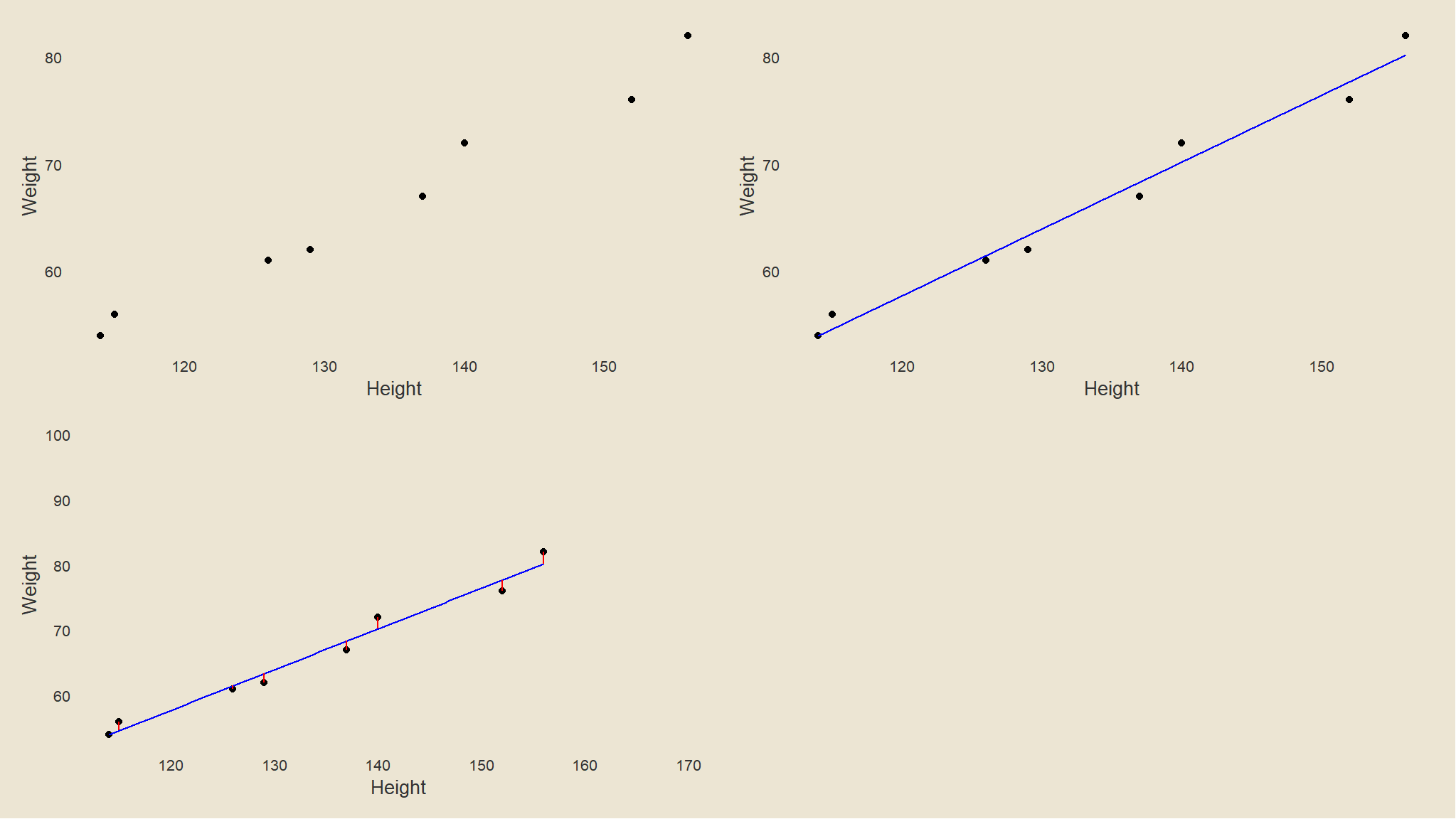

let us take the first five of these observations and use them to train a regression model.
In normal circustances you’d want to randomly split the data into training and validation sets + it is important for the split to be random to ensure that each subset is statistically similar

Splitting the data

# Split data into training and test sets
dummy_train_set <- df %>% 
  dplyr::slice(1:5)

dummy_test_set <- df %>% 
  dplyr::slice(6:8)

# Display the training set
dummy_train_set %>% 
  rename(c(x = Height, y = Weight)) %>% 
  flextable() %>%
  flextable::set_table_properties(width = .75, layout = "autofit") %>%
  flextable::theme_zebra() %>%
  flextable::fontsize(size = 12) %>%
  flextable::fontsize(size = 12, part = "header") %>%
  flextable::align_text_col(align = "center") %>%
  flextable::set_caption(caption = "")  %>%
  flextable::border_outer()

x	y
115	56
126	61
137	67
140	72
152	76

# Display the training set
theme_set(theme_light())
train_plot <- df %>%
  dplyr::slice(1:5) %>%
  rename(c(x = Height, y = Weight)) %>%
  ggplot(mapping = aes(x = x, y = y)) +
  geom_point(size = 1.6, color = "blue")+
  ylim(50, 80)+
  xlim(80, 160)+
  labs(x = 'x (Height)', y = 'y (Weight)')

train_plot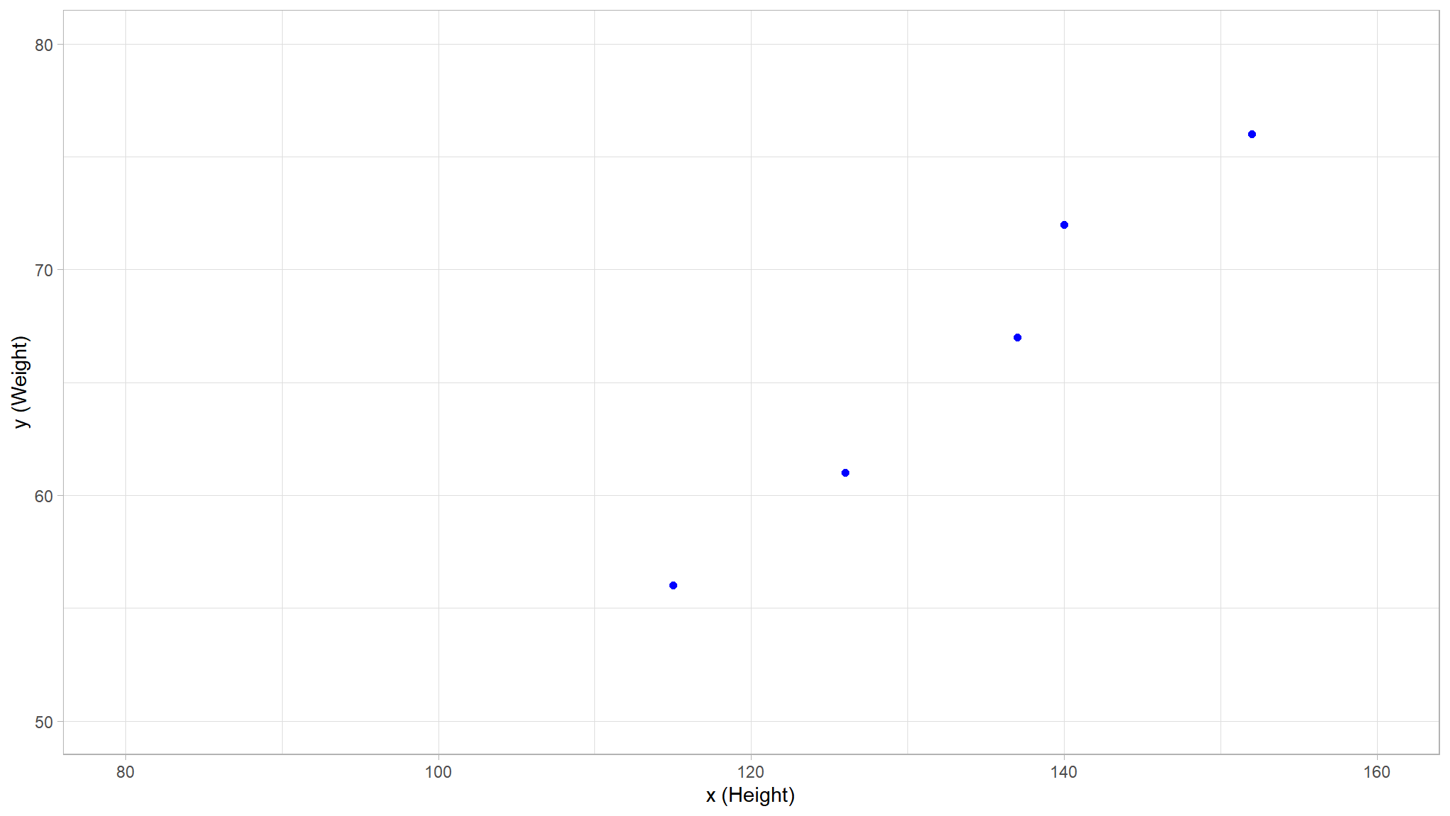

we note that there is some positive correlation between the two variables

You can probably see that the plotted points form an almost straight diagonal line
Now we need to fit these values to a function, allowing for some random variation.
in other words, there’s an apparent linearrelationship between $x$ and $y$, so we need to find a linear function that’s the best fit for the data sample.

let us plot a line a best fit (OLS method)

# Display the training set
theme_set(theme_light())
train_plot <- df %>%
  dplyr::slice(1:5) %>%
  rename(c(x = Height, y = Weight)) %>%
  ggplot(mapping = aes(x = x, y = y)) +
  geom_point(size = 1.6, color = "blue") +
  geom_smooth(method = 'lm', se = F, fullrange = TRUE, linetype = 3,
              color = "black", alpha = 0.2) +
  ggplot2::annotate("text", x = 140, y =70, label = "y =-6.16\ +\ 0.54x5", colour = "red")+
  ylim(50, 80)+
  xlim(80, 160)+
  labs(x = 'x (Temperature)', y = 'y (price)')

train_plot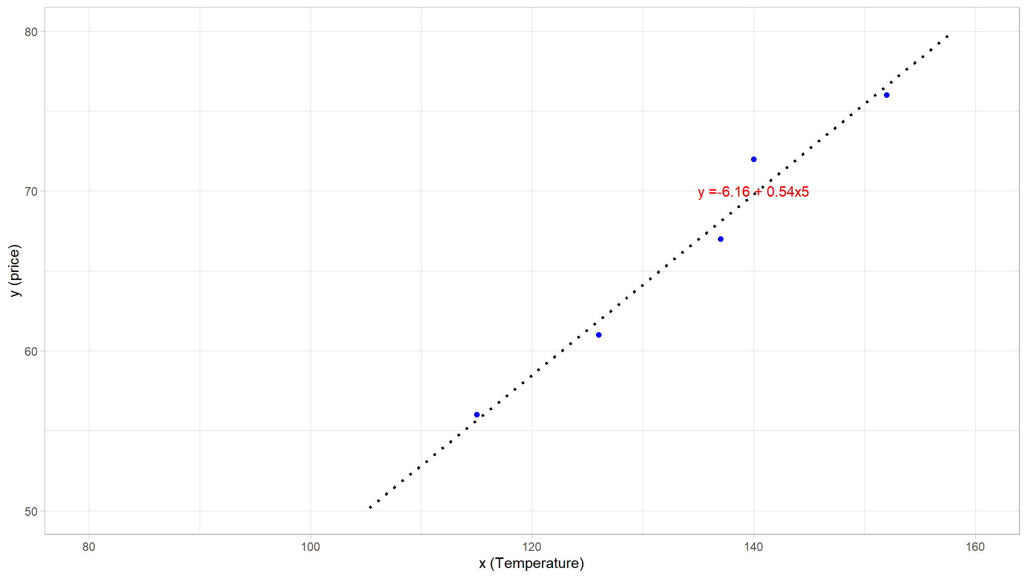

technically the line of best fit was fit using the Ordinary least squares method
lets examine a more a general equation of the line based on the points that lie exactly on the line . Recalling the equation of a straight line, because we assume that the expected relationship is linear, it will take the form:$y=mx+c$

Remember (from High school)

the equation of a straight line is given by $y=mx+c$ where

\[m=\frac{y_1-y_2}{x_1-x_2}\]

i will pick the obvious points (115,56) and (152,76) because they lie on the line of best fit

\[m=\frac{76-56}{152-115}\]

let’s do this in R

(76-56)/(152-115)
#> [1] 0.5405405

let’s solve for intercept

we know that $y=mx+c$ and we found m so $y-mx=c$

solving this using (115,56) in R we get

56-115*((76-56)/(152-115))
#> [1] -6.162162

this gives us the following function

\[ f(x) \ = \ -6.16\ +\ 0.54x \]

In this case, if we extended the line to the left we’d find that when $x$ is 0, $y$ is around -6.16, and the slope of the line is such that for each unit of $x$ you move along to the right, $y$ increases by around 0.54. Our $f$ function therefore can be calculated as:

\[ f(x) \ = \ -6.16\ +\ 0.54x \]

Now that we’ve defined ourpredictive function, we can use it to predict labels for the validation data we held back and compare the predicted values (which we typically indicate with the symbol $\hat y$, or “y-hat”) with the actual known $y$ values (Weight).

# Display the test set
dummy_test_set %>% 
  mutate("$\\hat{y}$" =(-6.16+0.54*Height)) %>% 
  knitr::kable()

Height	Weight	$\hat{y}$
156	82	78.08
114	54	55.40
129	62	63.50

Let’s see how the$\ y$ and $\hat y$ values compare in a plot:

# Make predictions using the linear model
dummy_pred <- dummy_test_set %>% 
  mutate("$\\hat{y}$" =(-6.16+0.54*Height))
colors <- c("Actual Weight" = "blue", "Predicted Weight" = "red")
# Comparison plot
dummy_pred_plot <- dummy_pred %>% 
  ggplot() +
  geom_point(aes(x = Height, y = Weight, color = "Actual Weight"))+
  geom_point(aes(x = Height, y = `$\\hat{y}$`, color = "Predicted Weight")) +
  geom_smooth(aes(x = Height, y = `$\\hat{y}$`), method = 'lm',se = F, fullrange = TRUE, linetype = 3, color = "black", alpha = 0.2) +
  ylim(50, 90)+
  xlim(80, 160)+
  labs(x = 'x (Height)', y = 'Weight' )+
  scale_color_manual(name = "",values = colors)

dummy_pred_plot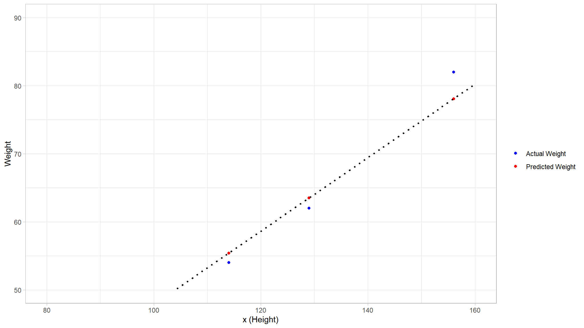

The plotted points that are on the function line are the predicted $\hat y$ values calculated by the function, and the other plotted points are the actual $y$ values.
There are various ways we can measure the variance between the predicted and actual values, and we can use these metrics to evaluate how well the model predicts.

You can think of the difference between a predicted label value and the actual label value as a measure of error. However, in practice, the “actual” values are based on sample observations (which themselves may be subject to some random variance). To make it clear that we’re comparing a predicted value ($\hat y$) with an observed value ($y$) we refer to the difference between them as the residuals. We can summarize the residuals for all of the validation data predictions to calculate the overall loss in the model as a measure of its predictive performance.

One of the most common ways to measure the loss is to square the individual residuals, sum the squares, and calculate the mean. Squaring the residuals has the effect of basing the calculation on absolute values (ignoring whether the difference is negative or positive) and giving more weight to larger differences. This metric is called the Mean Squared Error.

\[MSE= \frac{1}{n} \sum_{i=1}^{n} (y_i - \hat y_i)^2\] In other words, the MSE is the mean $\frac{1}{n}\sum_{i=1}^{n}$ of the squares of the errors $(y_i - \hat y_i)^2$

For our validation data, the calculation looks like this:

# Calculate residuals and square of residuals
dummy_mse <- dummy_test_set %>% 
  mutate("$\\hat{y}$" =(-6.16+0.54*Height)) %>% 
  select(-1) %>% 
  mutate("$y - \\hat{y}$ " = (.[1] - .[2])) %>% 
  mutate("$(y - \\hat{y})^2$ " = (.[3]^2)) %>% 
  rename("$y$" = 1)

dummy_mse %>% 
  knitr::kable()

$y$	$\hat{y}$	$y - \hat{y}$	$(y - \hat{y})^2$
82	78.08	3.92	15.3664
54	55.40	-1.40	1.9600
62	63.50	-1.50	2.2500

Great! Let’s go ahead and do some summary statistics on column $(y - \hat y)^2$ to obtain the total summation and the mean:

$\sum(y - \hat{y})^2$	$MSE$
19.5764	6.53

So the loss for our model based on the MSE metric is 6.53.

It’s difficult to tell whether this MSE value is good because it is not expressed in a meaningful unit of measurement.
However, we do know that the lower the value is, the less loss there is in the model; and therefore, the better it is predicting. This makes it a useful metric to compare two models and find the one that performs best.
Sometimes, it’s more useful to express the loss in the same unit of measurement as the predicted label value itself - in this case, the weight.
It’s possible to do this by calculating the square root of the MSE, which produces a metric known, unsurprisingly, as the Root Mean Squared Error (RMSE).

\[RMSE = \sqrt{9.79} = 2.56\]

So our model’s RMSE indicates that the loss is just over 2.5, which you can interpret loosely as meaning that on average, incorrect predictions are wrong by around 3 kgs of wight.

Multiple Linear Regression (Matrix form)

we can extend the above theory to multiple Regression i.e Regression with more than one independent variable
let us approach this using the Geometry of Least Squares

\[ \begin{aligned} \mathbf{\hat{y}} &= \mathbf{Xb} \\ &= \mathbf{X(X'X)^{-1}X'y} \\ &= \mathbf{Hy} \end{aligned} \]

sometimes H is denoted as P.

H is the projection operator.
\[ \mathbf{\hat{y}= Hy} \]

is the projection of y onto the linear space spanned by the columns of X (model space). The dimension of the model space is the rank of X.

Facts:

H is symmetric (i.e., H = H’)
HH = H

\[ \begin{aligned} \mathbf{HH} &= \mathbf{X(X'X)^{-1}X'X(X'X)^{-1}X'} \\ &= \mathbf{X(X'X)^{-1}IX'} \\ &= \mathbf{X(X'X)^{-1}X'} \end{aligned} \]

H is an n x n matrix with rank(H) = rank(X)
$\mathbf{(I-H) = I - X(X'X)^{-1}X'}$ is also a projection operator. It projects onto the n - k dimensional space that is orthogonal to the k dimensional space spanned by the columns of X
$\mathbf{H(I-H)=(I-H)H = 0}$

Partition of uncorrected total sum of squares:

\[ \begin{aligned} \mathbf{y'y} &= \mathbf{\hat{y}'\hat{y} + e'e} \\ &= \mathbf{(Hy)'(Hy) + ((I-H)y)'((I-H)y)} \\ &= \mathbf{y'H'Hy + y'(I-H)'(I-H)y} \\ &= \mathbf{y'Hy + y'(I-H)y} \\ \end{aligned} \]

or partition for the corrected total sum of squares:

\[ \mathbf{y'(I-H_1)y = y'(H-H_1)y + y'(I-H)y} \]

where $H_1 = \frac{1}{n} J = 1'(1'1)1$

Source	SS	df	MS	F
Regression	$SSR = \mathbf{y' (H-\frac{1}{n}J)y}$	p - 1	SSR/(p-1)	MSR /MSE
Error	$SSE = \mathbf{y'(I - H)y}$	n - p	SSE /(n-p)
Total	$\mathbf{y'y - y'Jy/n}$	n -1

Equivalently, we can express

\[ \mathbf{Y = X\hat{\beta} + (Y - X\hat{\beta})} \]

where

$\mathbf{\hat{Y} = X \hat{\beta}}$ = sum of a vector of fitted values
$\mathbf{e = ( Y - X \hat{\beta})}$ = residual
$\mathbf{Y}$ is the n x 1 vector in a n-dimensional space $R^n$
$\mathbf{X}$ is an n x p full rank matrix. and its columns generate a p-dimensional subspace of $R^n$. Hence, any estimator $\mathbf{X \hat{\beta}}$ is also in this subspace.

We choose least squares estimator that minimize the distance between $\mathbf{Y}$ and $\mathbf{X \hat{\beta}}$, which is the orthogonal projection of $\mathbf{Y}$ onto $\mathbf{X\beta}$.

\[ \begin{aligned} ||\mathbf{Y} - \mathbf{X}\hat{\beta}||^2 &= \mathbf{||Y - X\hat{\beta}||}^2 + \mathbf{||X \hat{\beta}||}^2 \\ &= \mathbf{(Y - X\hat{\beta})'(Y - X\hat{\beta}) +(X \hat{\beta})'(X \hat{\beta})} \\ &= \mathbf{(Y - X\hat{\beta})'Y - (Y - X\hat{\beta})'X\hat{\beta} + \hat{\beta}' X'X\hat{\beta}} \\ &= \mathbf{(Y-X\hat{\beta})'Y + \hat{\beta}'X'X(XX')^{-1}X'Y} \\ &= \mathbf{Y'Y - \hat{\beta}'X'Y + \hat{\beta}'X'Y} \end{aligned} \]

Normal Error Regression Model

\[ Y_i \sim N(\beta_0+\beta_1X_i, \sigma^2) \\ \]

$\beta_1$

Under the normal error model,

\[ b_1 \sim N(\beta_1,\frac{\sigma^2}{\sum_{i=1}^{n}(X_i - \bar{X})^2}) \]

A linear combination of independent normal random variable is normally distributed

Hence,

\[ \frac{b_1 - \beta_1}{s(b_1)} \sim t_{n-2} \]

A $(1-\alpha) 100 \%$ confidence interval for $\beta_1$ is

\[ b_1 \pm t_{t-\alpha/2 ; n-2}s(b_1) \]

$\beta_0$

Under the normal error model, the sampling distribution for $b_0$ is

\[ b_0 \sim N(\beta_0,\sigma^2(\frac{1}{n} + \frac{\bar{X}^2}{\sum_{i=1}^{n}(X_i - \bar{X})^2})) \]

Hence,

\[ \frac{b_0 - \beta_0}{s(b_0)} \sim t_{n-2} \] A $(1-\alpha)100 \%$ confidence interval for $\beta_0$ is

\[ b_0 \pm t_{1-\alpha/2;n-2}s(b_0) \]

Mean Response

Let $X_h$ denote the level of X for which we wish to estimate the mean response

We denote the mean response when $X = X_h$ by $E(Y_h)$
A point estimator of $E(Y_h)$ is $\hat{Y}_h$:

\[ \hat{Y}_h = b_0 + b_1 X_h \] Note

\[ E(\bar{Y}_h)= E(b_0 + b_1X_h) \\ = \beta_0 + \beta_1 X_h \\ = E(Y_h) \] (unbiased estimator)

\[ \begin{aligned} var(\hat{Y}_h) &= var(b_0 + b_1 X_h) \\ &= var(\hat{Y} + b_1 (X_h - \bar{X})) \\ &= var(\bar{Y}) + (X_h - \bar{X})^2var(b_1) + 2(X_h - \bar{X})cov(\bar{Y},b_1) \\ &= \frac{\sigma^2}{n} + (X_h - \bar{X})^2 \frac{\sigma^2}{\sum(X_i - \bar{X})^2} \\ &= \sigma^2(\frac{1}{n} + \frac{(X_h - \bar{X})^2}{\sum_{i=1}^{n} (X_i - \bar{X})^2}) \end{aligned} \]

Since $cov(\bar{Y},b_1) = 0$ due to the iid assumption on $\epsilon_i$

An estimate of this variance is

\[ s^2(\hat{Y}_h) = MSE (\frac{1}{n} + \frac{(X_h - \bar{X})^2}{\sum_{i=1}^{n}(X_i - \bar{X})^2}) \]

the sampling distribution for the mean response is

\[ \hat{Y}_h \sim N(E(Y_h),var(\hat{Y_h})) \\ \frac{\hat{Y}_h - E(Y_h)}{s(\hat{Y}_h)} \sim t_{n-2} \]

A $100(1-\alpha) \%$ CI for $E(Y_h)$ is

\[ \hat{Y}_h \pm t_{1-\alpha/2;n-2}s(\hat{Y}_h) \]

Prediction of a new observation

Regarding the Mean Response, we are interested in estimating mean of the distribution of Y given a certain X.

Now, we want to predict an individual outcome for the distribution of Y at a given X. We call $Y_{pred}$

Estimation of mean response versus prediction of a new observation:

the point estimates are the same in both cases: $\hat{Y}_{pred} = \hat{Y}_h$
It is the variance of the prediction that is different; hence, prediction intervals are different than confidence intervals. The prediction variance must consider:
- Variation in the mean of the distribution of Y
- Variation within the distribution of Y

We want to predict: mean response + error

\[ \beta_0 + \beta_1 X_h + \epsilon \]

Since $E(\epsilon) = 0$, use the least squares predictor:

\[ \hat{Y}_h = b_0 + b_1 X_h \]

The variance of the predictor is

\[ \begin{aligned} var(b_0 + b_1 X_h + \epsilon) &= var(b_0 + b_1 X_h) + var(\epsilon) \\ &= \sigma^2(\frac{1}{n} + \frac{(X_h - \bar{X})^2}{\sum_{i=1}^{n}(X_i - \bar{X})^2}) + \sigma^2 \\ &= \sigma^2(1+\frac{1}{n} + \frac{(X_h - \bar{X})^2}{\sum_{i=1}^{n}(X_i - \bar{X})^2}) \end{aligned} \]

An estimate of the variance is given by

\[ s^2(pred)= MSE (1+ \frac{1}{n} + \frac{(X_h - \bar{X})^2}{\sum_{i=1}^{n}(X_i - \bar{X})^2}) \\ \frac{Y_{pred}-\hat{Y}_h}{s(pred)} \sim t_{n-2} \]

$100(1-\alpha) \%$ prediction interval is

\[ \bar{Y}_h \pm t_{1-\alpha/2; n-2}s(pred) \]

The prediction interval is very sensitive to the distributional assumption on the errors, $\epsilon$

ANOVA

Partitioning the Total Sum of Squares: Consider the corrected Total sum of squares:

\[ SSTO = \sum_{i=1}^{n} (Y_i -\bar{Y})^2 \]

Measures the overall dispersion in the response variable
We use the term corrected because we correct for mean, the uncorrected total sum of squares is given by $\sum Y_i^2$

use $\hat{Y}_i = b_0 + b_1 X_i$ to estimate the conditional mean for Y at $X_i$

\[ \begin{aligned} \sum_{i=1}^n (Y_i - \bar{Y})^2 &= \sum_{i=1}^n (Y_i - \hat{Y}_i + \hat{Y}_i - \bar{Y})^2 \\ &= \sum_{i=1}^n(Y_i - \hat{Y}_i)^2 + \sum_{i=1}^n(\hat{Y}_i - \bar{Y})^2 + 2\sum_{i=1}^n(Y_i - \hat{Y}_i)(\hat{Y}_i-\bar{Y}) \\ &= \sum_{i=1}^n(Y_i - \hat{Y}_i)^2 + \sum_{i=1}^n(\bar{Y}_i -\bar{Y})^2 \\ STTO &= SSE + SSR \\ \end{aligned} \]

where SSR is the regression sum of squares, which measures how the conditional mean varies about a central value.

The cross-product term in the decomposition is 0:

\[ \begin{aligned} \sum_{i=1}^n (Y_i - \hat{Y}_i)(\hat{Y}_i - \bar{Y}) &= \sum_{i=1}^{n}(Y_i - \bar{Y} -b_1 (X_i - \bar{X}))(\bar{Y} + b_1 (X_i - \bar{X})-\bar{Y}) \\ &= b_1 \sum_{i=1}^{n} (Y_i - \bar{Y})(X_i - \bar{X}) - b_1^2\sum_{i=1}^{n}(X_i - \bar{X})^2 \\ &= b_1 \frac{\sum_{i=1}^{n}(Y_i -\bar{Y})(X_i - \bar{X})}{\sum_{i=1}^{n}(X_i - \bar{X})^2} \sum_{i=1}^{n}(X_i - \bar{X})^2 - b_1^2\sum_{i=1}^{n}(X_i - \bar{X})^2 \\ &= b_1^2 \sum_{i=1}^{n}(X_i - \bar{X})^2 - b_1^2 \sum_{i=1}^{n}(X_i - \bar{X})^2 \\ &= 0 \end{aligned} \]

\[ \begin{aligned} SSTO &= SSR + SSE \\ (n-1 d.f) &= (1 d.f.) + (n-2 d.f.) \end{aligned} \]

Source of Variation	Sum of Squares	df	Mean Square	F
Regression (model)	SSR	1	MSR = SSR/df	MSR/MSE
Error	SSE	n-2	MSE = SSE/df
Total (Corrected)	SSTO	n-1

\[ E(MSE) = \sigma^2 \\ E(MSR) = \sigma^2 + \beta_1^2 \sum_{i=1}^{n} (X_i - \bar{X})^2 \]

If $\beta_1 = 0$, then these two expected values are the same
if $\beta_1 \neq 0$ then E(MSR) will be larger than E(MSE)

which means the ratio of these two quantities, we can infer something about $\beta_1$

Distribution theory tells us that if $\epsilon_i \sim iid N(0,\sigma^2)$ and assuming $H_0: \beta_1 = 0$ is true,

\[ \frac{MSE}{\sigma^2} \sim \chi_{n-2}^2 \\ \frac{MSR}{\sigma^2} \sim \chi_{1}^2 \text{ if $\beta_1=0$} \]

where these two chi-square random variables are independent.

Since the ratio of 2 independent chi-square random variable follows an F distribution, we consider:

\[ F = \frac{MSR}{MSE} \sim F_{1,n-2} \]

when $\beta_1 =0$. Thus, we reject $H_0: \beta_1 = 0$ (or $E(Y_i)$ = constant) at $\alpha$ if

\[ F > F_{1 - \alpha;1,n-2} \]

this is the only null hypothesis that can be tested with this approach.

Coefficient of Determination

\[ R^2 = \frac{SSR}{SSTO} = 1- \frac{SSE}{SSTO} \]

where $0 \le R^2 \le 1$

Interpretation: The proportionate reduction of the total variation in Y after fitting a linear model in X.
It is not really correct to say that $R^2$ is the “variation in Y explained by X”.

$R^2$ is related to the correlation coefficient between Y and X:

\[ R^2 = (r)^2 \]

where $r= corr(x,y)$ is an estimate of the Pearson correlation coefficient. Also, note

\[ b_1 = (\frac{\sum_{i=1}^{n}(Y_i - \bar{Y})^2}{\sum_{i=1}^{n} (X_i - \bar{X})^2})^{1/2} \\ r = \frac{s_y}{s_x} r \]

Assumptions

Linearity of the regression function
Error terms have constant variance
Error terms are independent
No outliers
Error terms are normally distributed
No Omitted variables

Transformations

use transformations of one or both variables before performing the regression analysis.
The properties of least-squares estimates apply to the transformed regression, not the original variable.

If we transform the Y variable and perform regression to get:

\[ g(Y_i) = b_0 + b_1 X_i \]

Transform back:

\[ \hat{Y}_i = g^{-1}(b_0 + b_1 X_i) \]

$\hat{Y}_i$ will be biased. we can correct this bias.

Box-Cox Family Transformations

\[ Y'= Y^{\lambda} \]

where $\lambda$ is a parameter to be determined from the data.

$\lambda$	$Y'$
2	$Y^2$
0.5	$\sqrt{Y}$
0	$ln(Y)$
-0.5	$1/\sqrt{Y}$
-1	$1/Y$

To pick $\lambda$, we can do estimation by:

trial and error
maximum likelihood
numerical search

Case Study

read in the dataset

my_data<-readr::read_csv("airbnb_data.csv")
DT::datatable(my_data,filter="top")

What variables do we have

names(my_data)
#>  [1] "listing_id"         "description"        "host_id"           
#>  [4] "neighbourhood_full" "coordinates"        "room_type"         
#>  [7] "price"              "number_of_reviews"  "reviews_per_month" 
#> [10] "availability_365"   "rating"             "number_of_stays"   
#> [13] "listing_added"

How many observations do we have

dim(my_data)
#> [1] 7734   13

Do we have any missing values

colSums(is.na(my_data))
#>         listing_id        description            host_id neighbourhood_full 
#>                  0                  1                  7                  0 
#>        coordinates          room_type              price  number_of_reviews 
#>                  0                  0                  0                  0 
#>  reviews_per_month   availability_365             rating    number_of_stays 
#>                  0                  0                  0                  0 
#>      listing_added 
#>                  0

Let us look at the data clearly

glimpse(my_data)
#> Rows: 7,734
#> Columns: 13
#> $ listing_id         <dbl> 13740704, 22005115, 6425850, 22986519, 271954, 1421…
#> $ description        <chr> "Cozy,budget friendly, cable inc, private entrance!…
#> $ host_id            <dbl> 20583125, 82746113, 32715865, 154262349, 1423798, 7…
#> $ neighbourhood_full <chr> "Brooklyn, Flatlands", "Manhattan, Upper West Side"…
#> $ coordinates        <chr> "(40.63222, -73.93398)", "(40.78761, -73.96862)", "…
#> $ room_type          <chr> "Private Room", "Entire place", "Entire place", "Pr…
#> $ price              <dbl> 45, 135, 86, 160, 150, 224, 169, 75, 50, 254, 41, 9…
#> $ number_of_reviews  <dbl> 10, 1, 5, 23, 203, 2, 5, 8, 5, 2, 21, 94, 6, 90, 5,…
#> $ reviews_per_month  <dbl> 0.70, 1.00, 0.13, 2.29, 2.22, 0.08, 0.15, 0.66, 0.4…
#> $ availability_365   <dbl> 85, 145, 0, 102, 300, 353, 365, 9, 0, 24, 334, 117,…
#> $ rating             <dbl> 4.100954, 3.367600, 4.763203, 3.822591, 4.478396, 4…
#> $ number_of_stays    <dbl> 12.0, 1.2, 6.0, 27.6, 243.6, 2.4, 6.0, 9.6, 6.0, 2.…
#> $ listing_added      <date> 2018-06-08, 2018-12-25, 2017-03-20, 2020-10-23, 20…

Lets look at anormalies in the variables

my_data |> 
  janitor::tabyl(room_type)
#>     room_type    n    percent
#>  Entire place 4075 0.52689423
#>  Private Room 3494 0.45177140
#>   Shared room  165 0.02133437

my_data |> 
  janitor::tabyl(neighbourhood_full) |> 
  as_tibble() |> 
  arrange(desc(n))
#> # A tibble: 192 × 3
#>    neighbourhood_full               n percent
#>    <chr>                        <int>   <dbl>
#>  1 Brooklyn, Bedford-Stuyvesant   636  0.0822
#>  2 Brooklyn, Williamsburg         609  0.0787
#>  3 Manhattan, Harlem              441  0.0570
#>  4 Brooklyn, Bushwick             373  0.0482
#>  5 Manhattan, Hell's Kitchen      305  0.0394
#>  6 Manhattan, East Village        290  0.0375
#>  7 Manhattan, Upper West Side     290  0.0375
#>  8 Manhattan, Upper East Side     282  0.0365
#>  9 Brooklyn, Crown Heights        255  0.0330
#> 10 Manhattan, Midtown             212  0.0274
#> # ℹ 182 more rows

that is way too many categories to work with
we will visualise the most listed neighborhoods

Top 20 most listed neighborhoods

my_data |> 
  janitor::tabyl(neighbourhood_full) |> 
  as_tibble() |> 
  arrange(desc(n)) |> 
  head(20) |> 
  mutate(neighbourhood_ful=fct_reorder(neighbourhood_full, n)) |>
  ggplot(aes(x=fct_reorder(neighbourhood_full, n), n)) +
  geom_col() + 
  scale_fill_avatar()+
  theme_avatar()+
  labs(x="Neighborhood", 
       y="count", 
       title="Top 20 most listed Neighhoods") + 
  coord_flip() + 
  geom_text(aes(label=paste0(round(n), "x "), hjust=1), col="white")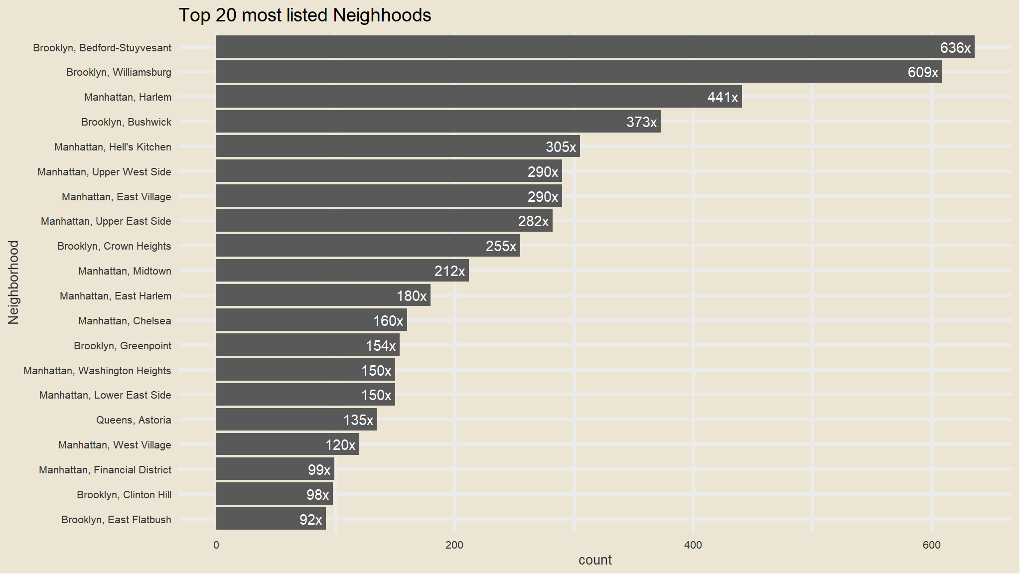

Data Wrangling

we will just categorise the neighborhoods into 4 categories
the initial looking at neighbourhood_full we note that the observations have the values with initial texts have 5 categories

out_new<-my_data |> 
  mutate(neighbourhood_location=
           case_when(str_detect(neighbourhood_full,"Staten Island")~"Staten Island",
                     str_detect(neighbourhood_full,"Queens")~"Queens",
                     str_detect(neighbourhood_full,"Manhattan")~"Manhattan",
                     str_detect(neighbourhood_full,"Brooklyn")~"Brooklyn",
                     str_detect(neighbourhood_full,"Bronx")~"Bronx"))

Count of neighborhoods

out_new |> 
  janitor::tabyl(neighbourhood_location) |> 
  as_tibble() |> 
  arrange(desc(n)) |> 
  ggplot(aes(x=fct_reorder(neighbourhood_location, n), n)) +
  geom_col() + 
  scale_fill_avatar()+
  theme_avatar()+
  labs(x="Neighborhood", 
       y="count", 
       title="") + 
  coord_flip() + 
  geom_text(aes(label=paste0(round(n), "x "), hjust=1), col="purple")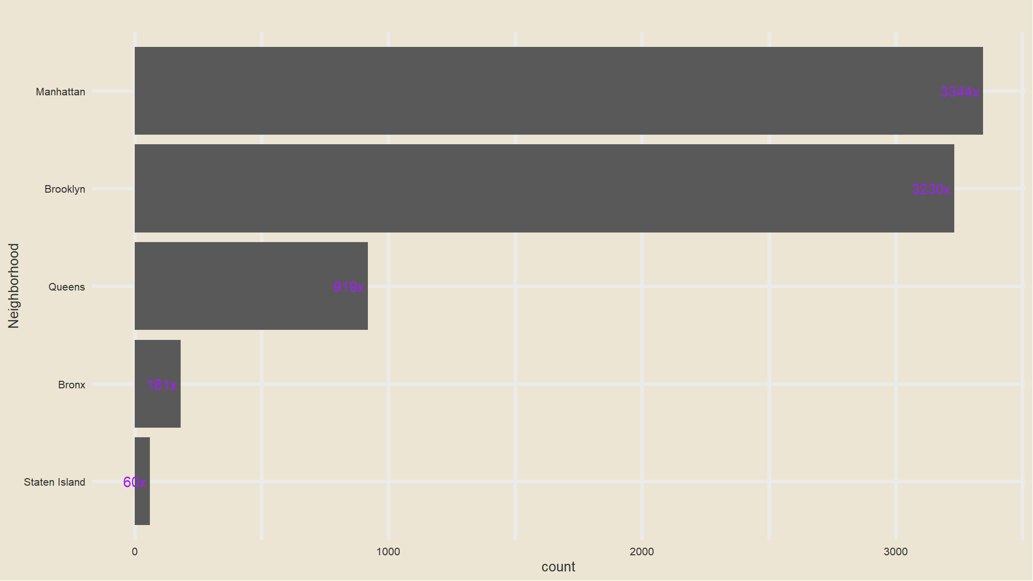

Note

Comments

that is now better , we seem to have managable categories now.
Manhattan has the greatest number of listings

Mean Price comparison in Each neighborhood

out_new |> 
  group_by(neighbourhood_location) |> 
  summarise(avg=mean(price)) |> 
  ggplot(aes(x=fct_reorder(neighbourhood_location, avg), avg)) +
  geom_col() + 
  scale_fill_avatar()+
  theme_avatar()+
  labs(x="Neighborhood", 
       y="Average", 
       title="") + 
  coord_flip() + 
  geom_text(aes(label=paste0(round(avg), "$"), hjust=1), col="purple")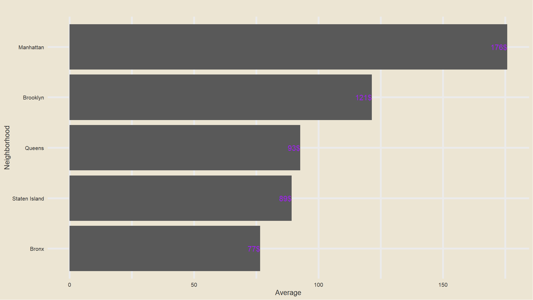

Note

Comments

average price listings is highest in Manhattan followed by Brooklyn this could be due to the fact that the most common type of listings is the entire apartment
Bronx Has the cheapest listings as compared to others

Mean Price comparison in Each room type

out_new |> 
  group_by(room_type) |> 
  summarise(avg=mean(price)) |> 
  ggplot(aes(x=fct_reorder(room_type, avg), avg)) +
  geom_col() + 
  scale_fill_avatar()+
  theme_avatar()+
  labs(x="Room Type", 
       y="Average", 
       title="") + 
  coord_flip() + 
  geom_text(aes(label=paste0(round(avg), "$"), hjust=1), col="purple")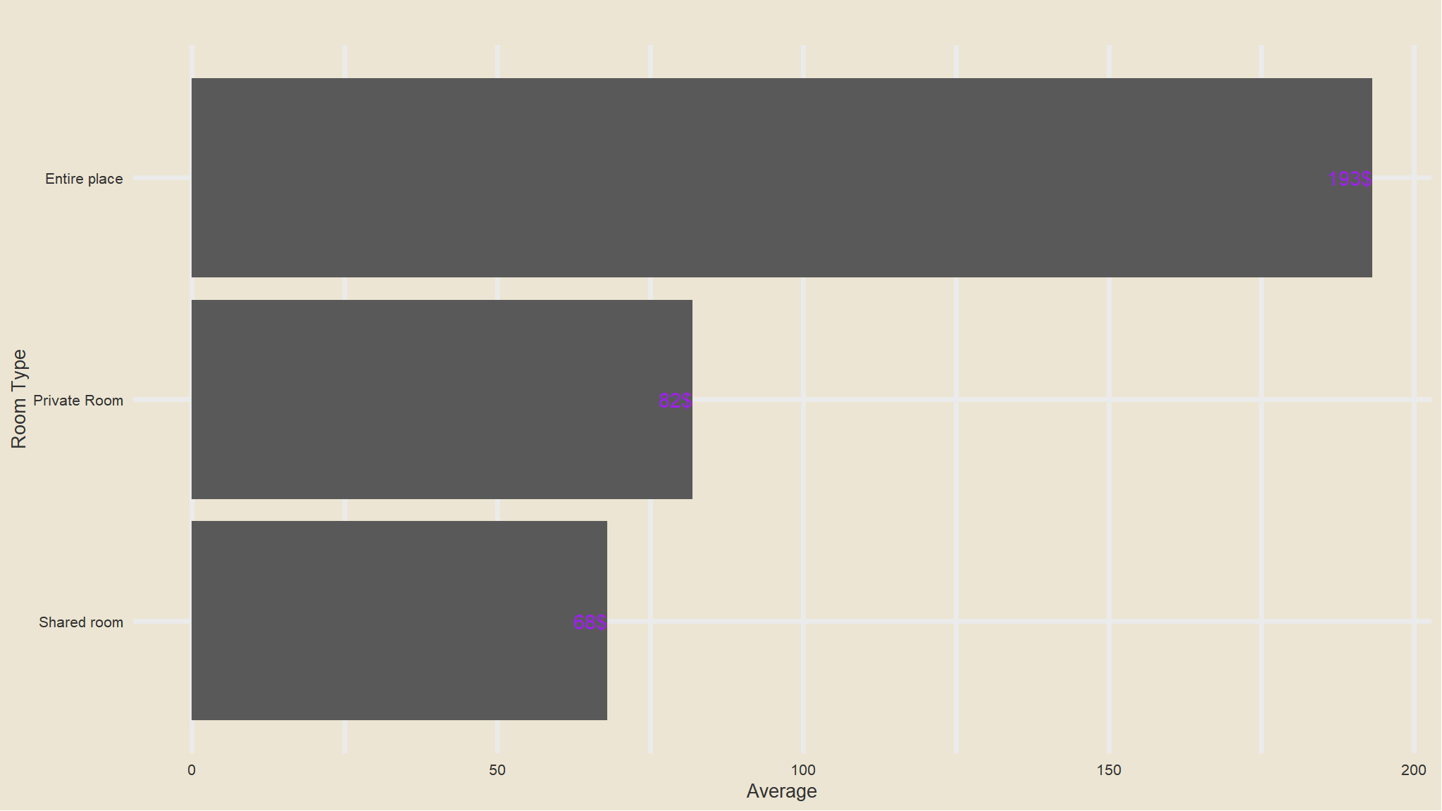

Note

Comments

Whole apartments have the largest prices compared to other rooms , this is really expected

Geospatial data

out_new |> 
  relocate(coordinates)
#> # A tibble: 7,734 × 14
#>    coordinates listing_id description host_id neighbourhood_full room_type price
#>    <chr>            <dbl> <chr>         <dbl> <chr>              <chr>     <dbl>
#>  1 (40.63222,…   13740704 Cozy,budge…  2.06e7 Brooklyn, Flatlan… Private …    45
#>  2 (40.78761,…   22005115 Two floor …  8.27e7 Manhattan, Upper … Entire p…   135
#>  3 (40.79169,…    6425850 Spacious, …  3.27e7 Manhattan, Upper … Entire p…    86
#>  4 (40.71884,…   22986519 Bedroom on…  1.54e8 Manhattan, Lower … Private …   160
#>  5 (40.73388,…     271954 Beautiful …  1.42e6 Manhattan, Greenw… Entire p…   150
#>  6 (40.58531,…   14218742 Luxury/3be…  7.88e7 Brooklyn, Sheepsh… Entire p…   224
#>  7 (40.761, -…   15125599 Beautiful …  3.19e6 Manhattan, Theate… Entire p…   169
#>  8 (40.80667,…   24553891 Enjoy all …  6.86e7 Manhattan, Harlem  Entire p…    75
#>  9 (40.70103,…   26386759 Cozy and e…  8.69e7 Brooklyn, Bushwick Private …    50
#> 10 (40.6688, …   34446664 Home away …  2.60e8 Queens, Laurelton  Entire p…   254
#> # ℹ 7,724 more rows
#> # ℹ 7 more variables: number_of_reviews <dbl>, reviews_per_month <dbl>,
#> #   availability_365 <dbl>, rating <dbl>, number_of_stays <dbl>,
#> #   listing_added <date>, neighbourhood_location <chr>

out_new |> 
  separate(coordinates,into=c("lAT","LONG"),sep=",") |> 
  relocate(lAT,LONG)
#> # A tibble: 7,734 × 15
#>    lAT   LONG  listing_id description host_id neighbourhood_full room_type price
#>    <chr> <chr>      <dbl> <chr>         <dbl> <chr>              <chr>     <dbl>
#>  1 (40.… " -7…   13740704 Cozy,budge…  2.06e7 Brooklyn, Flatlan… Private …    45
#>  2 (40.… " -7…   22005115 Two floor …  8.27e7 Manhattan, Upper … Entire p…   135
#>  3 (40.… " -7…    6425850 Spacious, …  3.27e7 Manhattan, Upper … Entire p…    86
#>  4 (40.… " -7…   22986519 Bedroom on…  1.54e8 Manhattan, Lower … Private …   160
#>  5 (40.… " -7…     271954 Beautiful …  1.42e6 Manhattan, Greenw… Entire p…   150
#>  6 (40.… " -7…   14218742 Luxury/3be…  7.88e7 Brooklyn, Sheepsh… Entire p…   224
#>  7 (40.… " -7…   15125599 Beautiful …  3.19e6 Manhattan, Theate… Entire p…   169
#>  8 (40.… " -7…   24553891 Enjoy all …  6.86e7 Manhattan, Harlem  Entire p…    75
#>  9 (40.… " -7…   26386759 Cozy and e…  8.69e7 Brooklyn, Bushwick Private …    50
#> 10 (40.… " -7…   34446664 Home away …  2.60e8 Queens, Laurelton  Entire p…   254
#> # ℹ 7,724 more rows
#> # ℹ 7 more variables: number_of_reviews <dbl>, reviews_per_month <dbl>,
#> #   availability_365 <dbl>, rating <dbl>, number_of_stays <dbl>,
#> #   listing_added <date>, neighbourhood_location <chr>

interesting , note that i am doing this the easisest and most understandable way

next up i need to remove the brackets and save the whole thing into an object

out_new<-out_new |> 
  separate(coordinates,into=c("lAT","LONG"),sep=",") |> 
  relocate(lAT,LONG) |> 
  mutate(lAT=readr::parse_number(lAT),
         LONG=readr::parse_number(LONG))
out_new
#> # A tibble: 7,734 × 15
#>      lAT  LONG listing_id description host_id neighbourhood_full room_type price
#>    <dbl> <dbl>      <dbl> <chr>         <dbl> <chr>              <chr>     <dbl>
#>  1  40.6 -73.9   13740704 Cozy,budge…  2.06e7 Brooklyn, Flatlan… Private …    45
#>  2  40.8 -74.0   22005115 Two floor …  8.27e7 Manhattan, Upper … Entire p…   135
#>  3  40.8 -74.0    6425850 Spacious, …  3.27e7 Manhattan, Upper … Entire p…    86
#>  4  40.7 -74.0   22986519 Bedroom on…  1.54e8 Manhattan, Lower … Private …   160
#>  5  40.7 -74.0     271954 Beautiful …  1.42e6 Manhattan, Greenw… Entire p…   150
#>  6  40.6 -73.9   14218742 Luxury/3be…  7.88e7 Brooklyn, Sheepsh… Entire p…   224
#>  7  40.8 -74.0   15125599 Beautiful …  3.19e6 Manhattan, Theate… Entire p…   169
#>  8  40.8 -74.0   24553891 Enjoy all …  6.86e7 Manhattan, Harlem  Entire p…    75
#>  9  40.7 -73.9   26386759 Cozy and e…  8.69e7 Brooklyn, Bushwick Private …    50
#> 10  40.7 -73.7   34446664 Home away …  2.60e8 Queens, Laurelton  Entire p…   254
#> # ℹ 7,724 more rows
#> # ℹ 7 more variables: number_of_reviews <dbl>, reviews_per_month <dbl>,
#> #   availability_365 <dbl>, rating <dbl>, number_of_stays <dbl>,
#> #   listing_added <date>, neighbourhood_location <chr>

library(viridis)
ggplot(out_new, aes(LONG, lAT,fill=neighbourhood_location)) +
  geom_point(
    alpha = 1,
    shape = 21,
    colour = "black",
    size = 5,
    position = "jitter"
  ) +
  scale_fill_viridis(
    discrete = TRUE,
    name = ""
  ) +
  ggtitle("Figure 3: look at the locations and geocodes ") +
  ylab("Latitude") +
  xlab("Longitude")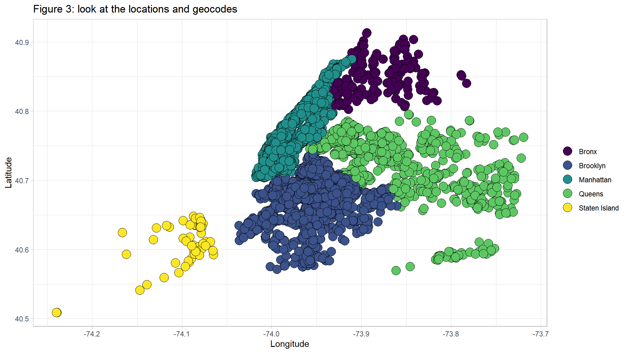

ggplot(out_new, aes(LONG, lAT)) +
  geom_point(aes(color=price)) +
  scale_color_gradient(low="blue",high="red") +
  facet_wrap(~neighbourhood_location,scales="free")+
  ggtitle("Figure 4: distribution of prices? ") +
  ylab("Latitude") +
  xlab("Longitude")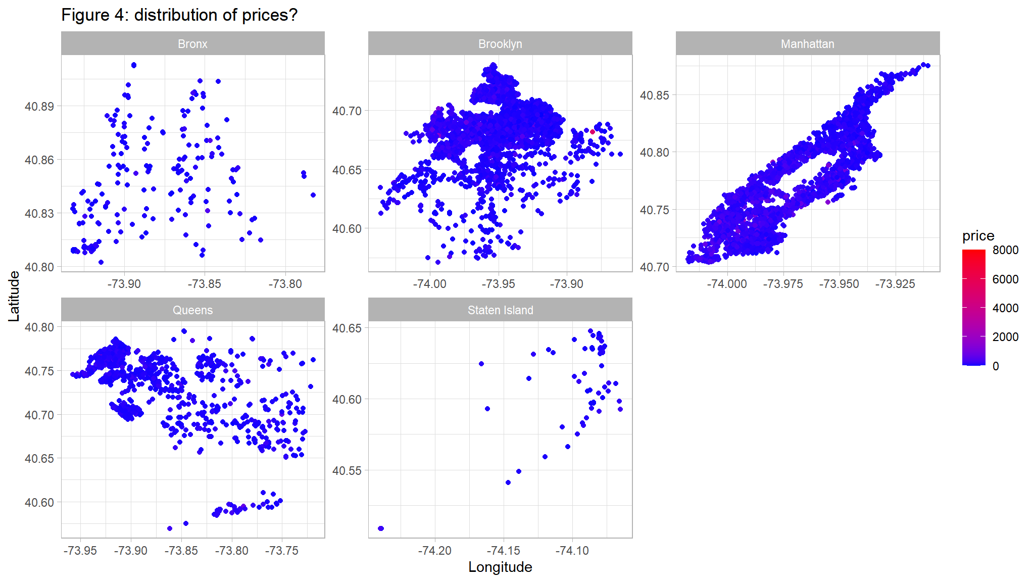


ggplot(out_new, aes(LONG, lAT)) +
  geom_point(aes(color=number_of_reviews)) +
  scale_color_gradient(low="blue",high="red") +
  facet_wrap(~neighbourhood_location,scales="free")+
  ggtitle("Figure 4: distribution of reviews ") +
  ylab("Latitude") +
  xlab("Longitude")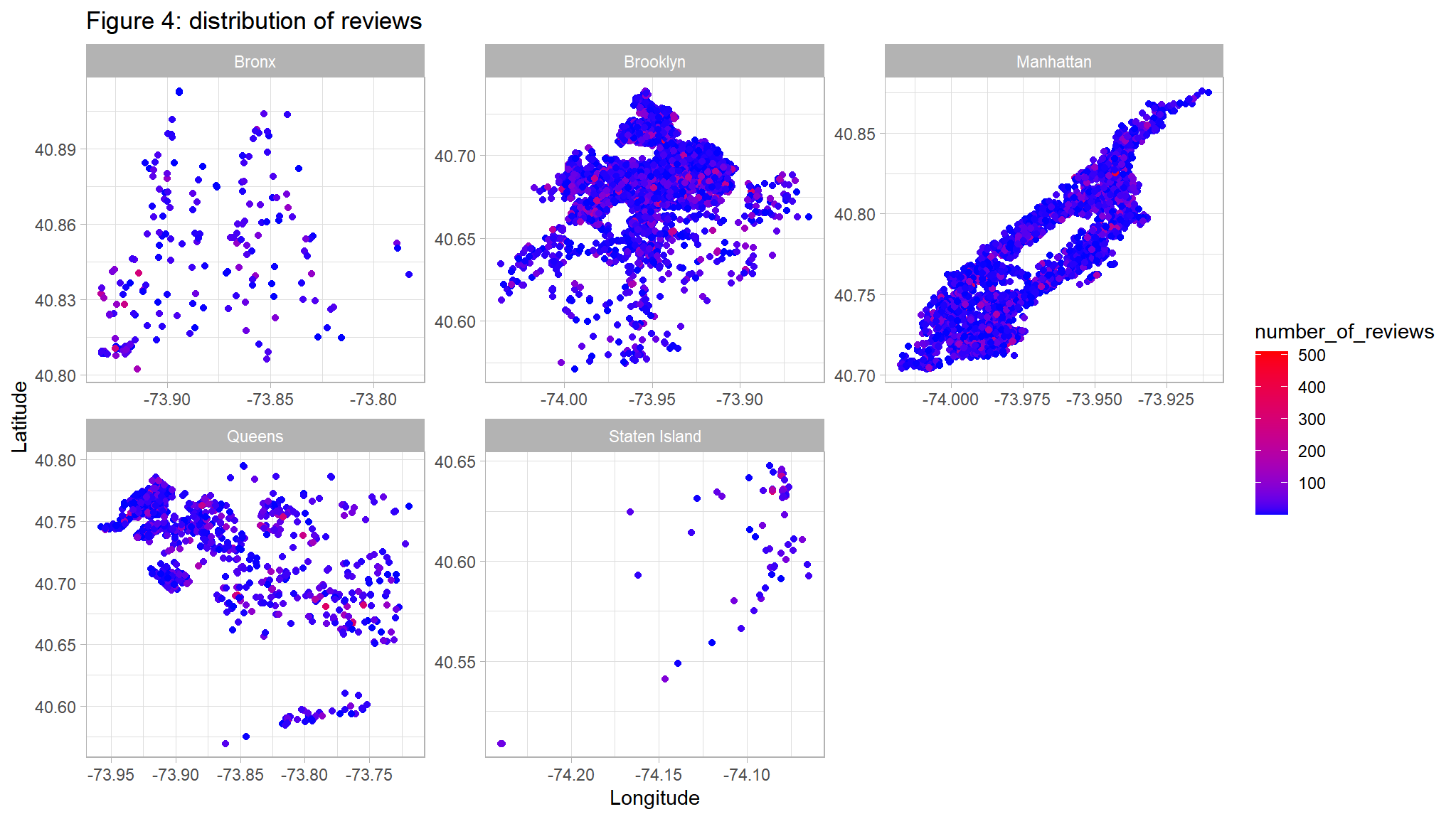

ggplot(out_new, aes(LONG, lAT,color=room_type)) +
  geom_point() +
  facet_wrap(~neighbourhood_location,scales="free")+
  ggtitle("Figure 4: distribution of room type by location") +
  ylab("Latitude") +
  xlab("Longitude")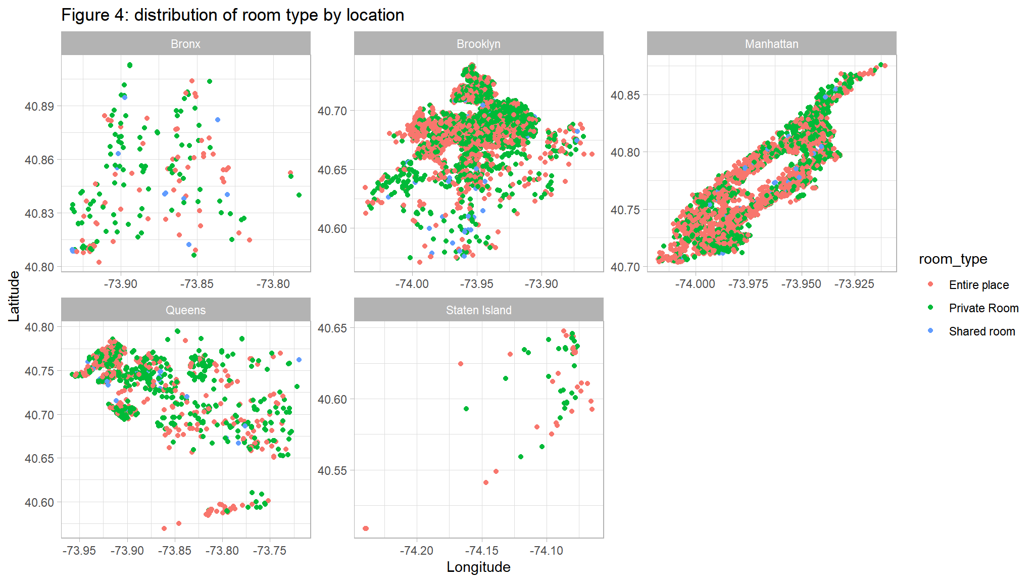

distribution of numeric data

out_new |> 
  select_if(is.numeric) |> 
  select(-LONG,-lAT,-host_id,-listing_id) |> 
  gather("features","values") |>
  group_by(features) |> 
  mutate(Mean = mean(values),
         Median = median(values)) |>
  ggplot(aes(x=values,fill=features))+
  geom_histogram()+
  facet_wrap(~features,scales="free")+
  tvthemes::scale_fill_avatar() +
  # Add lines for mean and median
  geom_vline(aes(xintercept = Mean, color = "Mean"), linetype = "dashed", size = 1.3 ) +
  geom_vline(aes(xintercept = Median, color = "Median"), linetype = "dashed", size = 1.3 ) +
  scale_color_manual(name = "", values = c(Mean = "red", Median = "yellow"))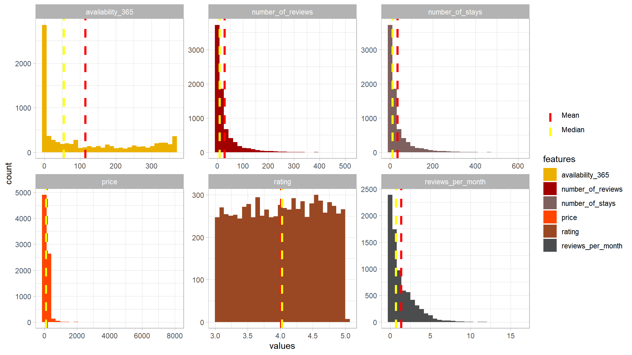

out_new |> 
  select_if(is.numeric) |> 
  select(-LONG,-lAT,-host_id,-listing_id) |> 
  gather() |> 
  ggplot(aes(y=value,x=key,fill=key))+
  geom_boxplot()+
  facet_wrap(~key,scales="free")+
  tvthemes::scale_fill_avatar()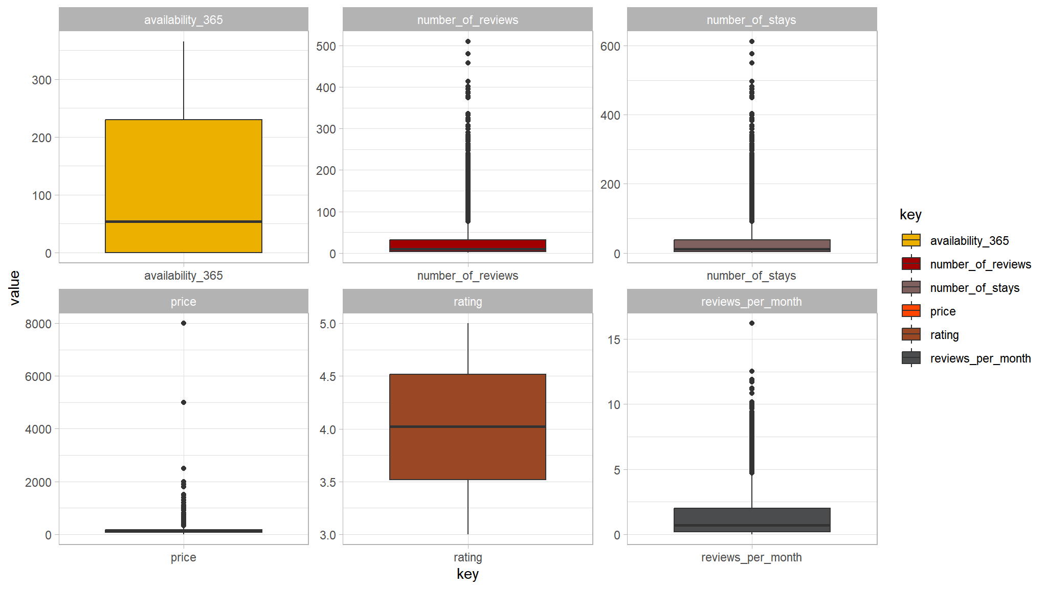

the variable price seems to have a couple of outliers in it
attempt to remove all values greater than 2000

out_new |> 
  select_if(is.numeric) |> 
  dplyr::filter(price<2000) |> 
  select(-LONG,-lAT,-host_id,-listing_id) |> 
  gather() |> 
  ggplot(aes(y=value,x=key,fill=key))+
  geom_boxplot()+
  facet_wrap(~key,scales="free")+
  tvthemes::scale_fill_avatar()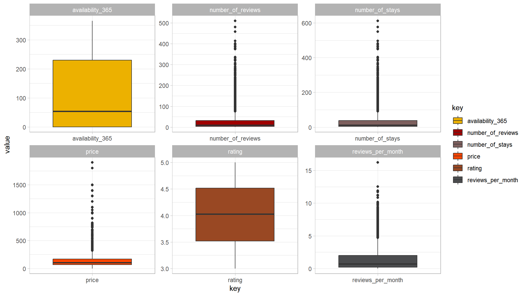

not so bad after all , we will take this into consideration while modeling


# Plot a scatter plot for each feature
out_new |> 
  select_if(is.numeric) |> 
  select(-host_id,-listing_id) |> 
  gather("features","values",-price) |>
  group_by(features) |> 
  mutate(Mean = mean(values),
         Median = median(values)) |> 
  mutate(corr_coef = cor(values, price)) |> 
  mutate(features = paste(features, ' vs price, r = ', corr_coef, sep = '')) |> 
  ggplot(aes(x = values, y = price, color = features)) +
  geom_point(alpha = 0.7, show.legend = F) +
  facet_wrap(~ features, scales = 'free')+
  paletteer::scale_color_paletteer_d("ggthemes::excel_Parallax")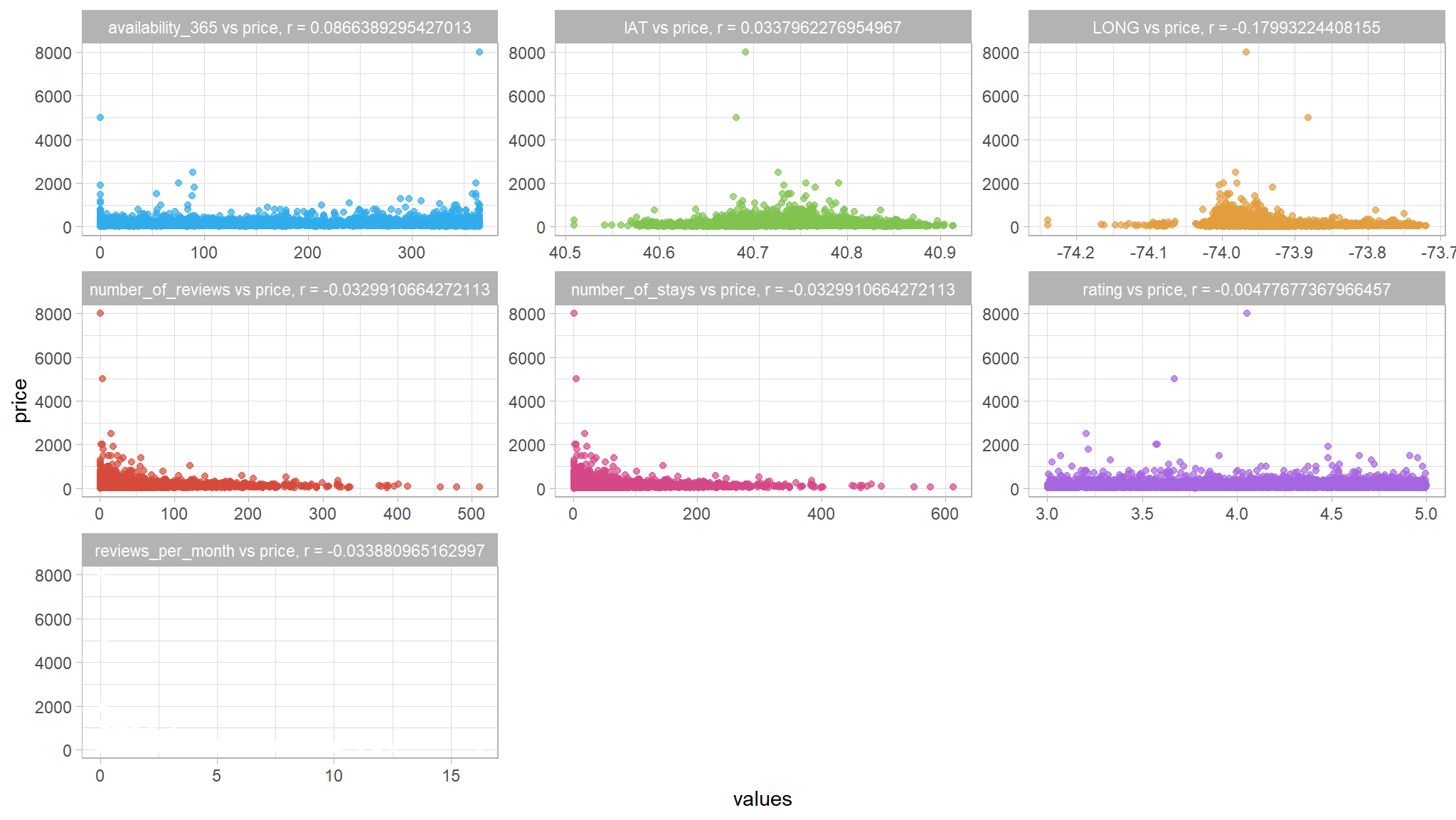

we dont see any type of correlation within the data

room type by neighhood

ggplot(out_new) +                             # data to use 
  aes(x=room_type) +                                        # x = predictor  (factor) 
  aes(fill=room_type) +                                         # fill = outcome (factor)  
  geom_bar( position="dodge",                                        # side-by-side  
       color="black") +                                                  # choose color of bar borders 
    tvthemes::scale_color_kimPossible() +       # choose colors of bars 
    tvthemes::scale_fill_avatar()  +   # bars 
  geom_text(aes(label=after_stat(count)),                    # required  
     stat='count',                                           # required 
     position=position_dodge(1.0),                           # required for centering  
     vjust= -0.5, 
     size=3) + 
   scale_x_discrete(limits = rev) +                                       # reverse order to 0 cups first 
   # FORCE y-axis ticks 
  facet_grid(~ neighbourhood_location)  +                                              # Strata in 1 row 
  ggtitle("room type, neighbhourhood \nStratified") +           # title and axis labels 
  xlab("") +  
  ylab("Count") + 
  theme_bw() + 
  theme(legend.title=element_blank()) + 
  theme(legend.text=element_text(color="black", size=6)) + 
  theme(legend.position="right") +
  theme(axis.text.x = element_text(angle = 45, hjust = 1))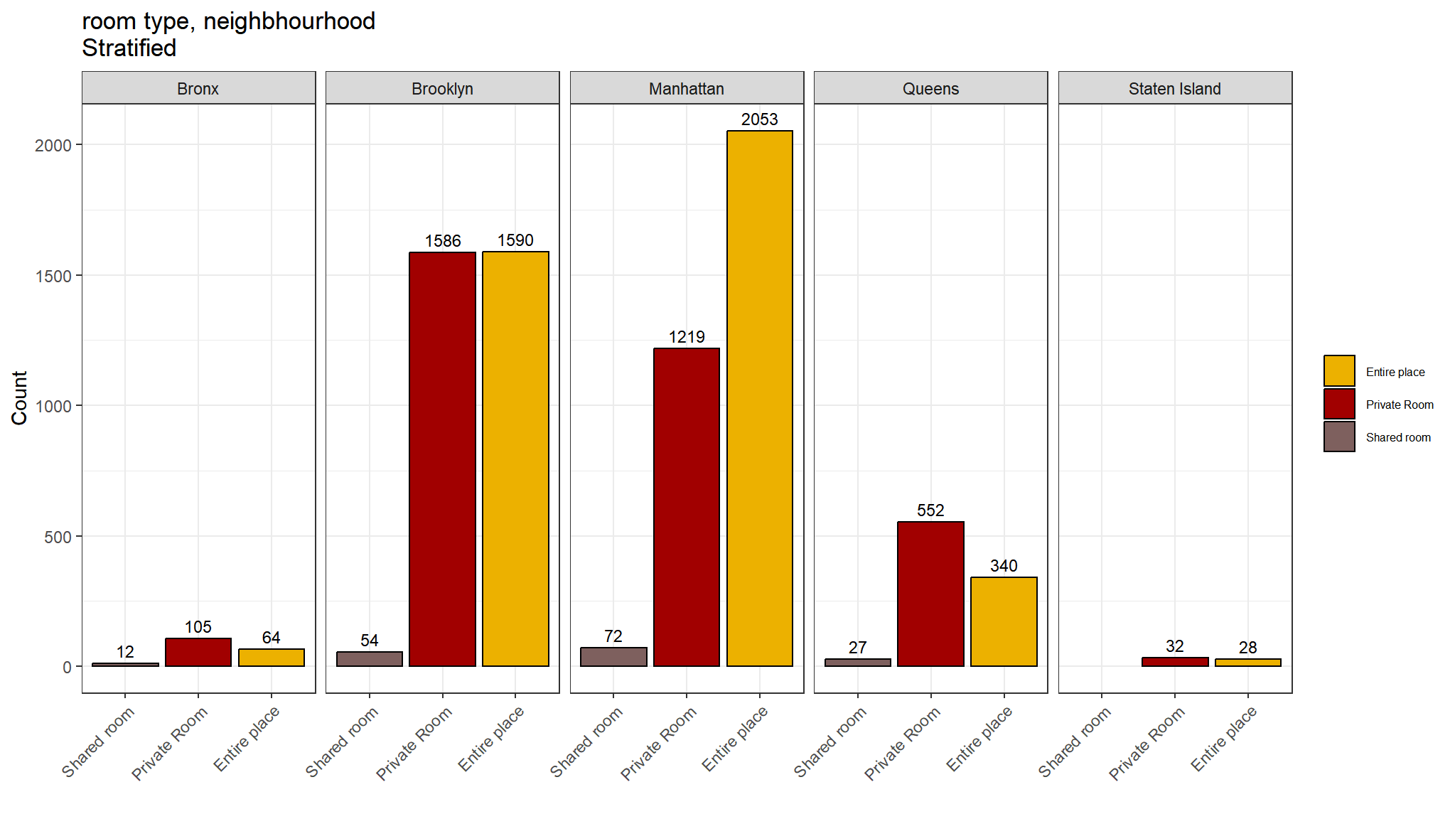

Note

Comments

Private rooms are the most common listing type in most neighbourhoods
However in Manhattan Entire place is the most commontype
Shared rooms are least common

correlations

## select only numeric values
cor_data<-out_new|> 
  select_if(is.numeric) |> 
  select(-host_id,-listing_id)
  
## create a correlation matrix
corl<-cor(cor_data)
corrplot::corrplot(corl,method="color",addCoef.col = "black")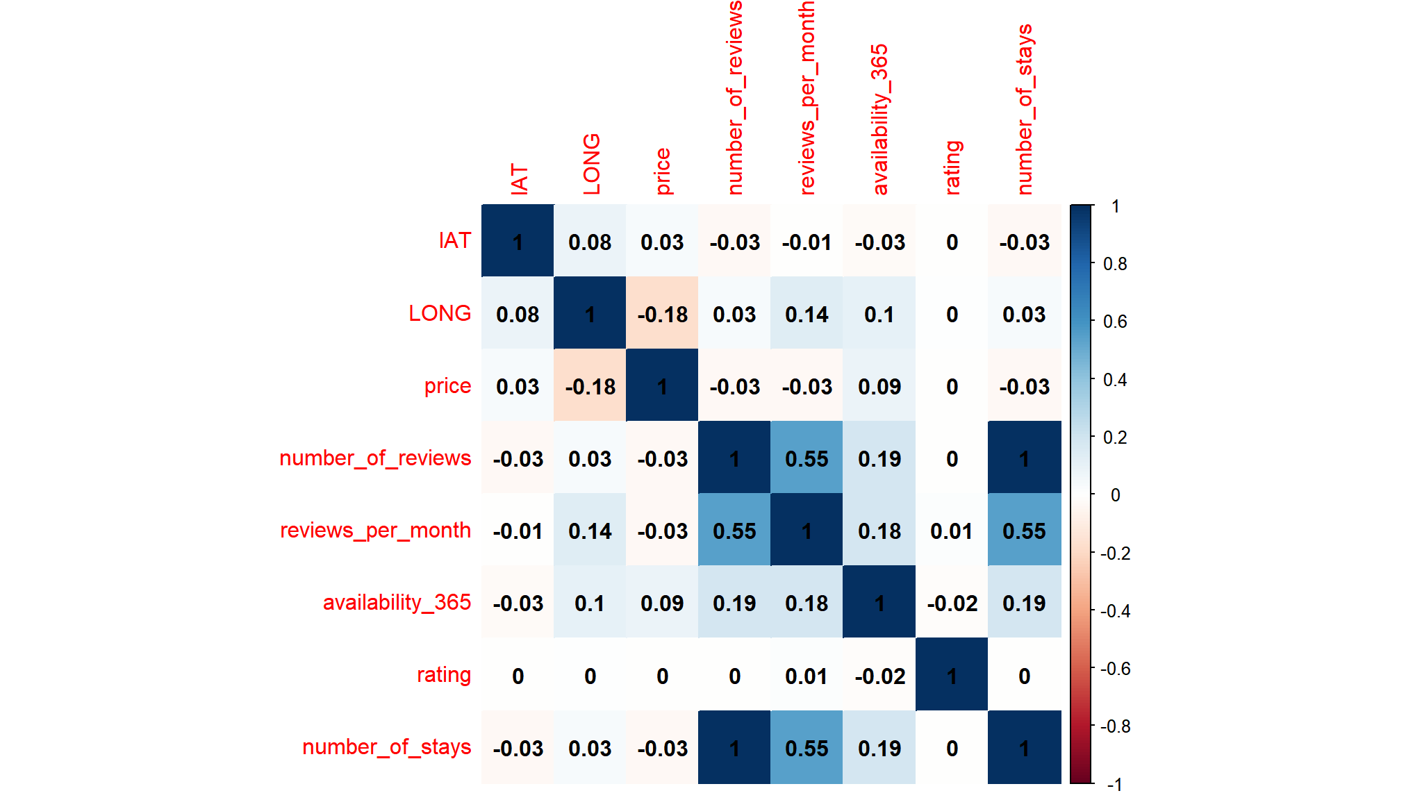

there is a strong positive correlation between number of stays and number of reviews
the correlation is 1 so we are going to remove number of reviews as will cause problems in our model

summary statistics

out_new |> 
  select_if(is.numeric) |> 
  select(-LONG,-lAT,-host_id,-listing_id) |> 
  # Summary stats
  descr(order = "preserve",
        stats = c('mean', 'sd', 'min', 'q1', 'med', 'q3', 'max'),
        round.digits = 6)
#> Descriptive Statistics  
#> 
#>                       price   number_of_reviews   reviews_per_month   availability_365     rating
#> ------------- ------------- ------------------- ------------------- ------------------ ----------
#>          Mean    140.244375           28.355185            1.353746         114.546160   4.012199
#>       Std.Dev    163.769252           46.962275            1.613229         129.862583   0.574812
#>           Min      0.000000            1.000000            0.010000           0.000000   3.000633
#>            Q1     69.000000            3.000000            0.200000           0.000000   3.518917
#>        Median    105.000000            9.000000            0.710000          54.000000   4.024223
#>            Q3    170.000000           32.000000            2.000000         230.000000   4.514260
#>           Max   8000.000000          510.000000           16.220000         365.000000   4.999561
#> 
#> Table: Table continues below
#> 
#>  
#> 
#>                 number_of_stays
#> ------------- -----------------
#>          Mean         34.026222
#>       Std.Dev         56.354729
#>           Min          1.200000
#>            Q1          3.600000
#>        Median         10.800000
#>            Q3         38.400000
#>           Max        612.000000

as noted earlier ,prices around 8000 seems to me as outliers , so i have chosen a cutoff point of 2000

Prepare data for modeling

cases<-complete.cases(out_new)
out_new_data<-out_new[cases,]
out_new_data<-out_new_data |> 
  dplyr::filter(price<2000) |> 
  select(-host_id,-listing_id,-neighbourhood_full,-listing_added,-description,-number_of_reviews,-lAT,-LONG) |> 
  mutate_if(is.character,as.factor)

Building a Regression Model

# Load the Tidymodels packages
library(tidymodels)

# Split 70% of the data for training and the rest for tesing
set.seed(2056)
abnb_split <- out_new_data %>% 
  initial_split(prop = 0.7,
  # splitting data evenly on the holiday variable
                strata = price)

# Extract the data in each split
abnb_train <- training(abnb_split)
abnb_test <- testing(abnb_split)

glue::glue(
  'Training Set: {nrow(abnb_train)} rows
  Test Set: {nrow(abnb_test)} rows')
#> Training Set: 5403 rows
#> Test Set: 2318 rows

Tip

This results into the following two datasets:

abnb_train: subset of the dataset used to train the model.
abnb_test: subset of the dataset used to validate the model.

Note

In Tidymodels, you specify models using parsnip(). The goal of parsnip is to provide a tidy, unified interface to models that can be used to try a range of models by specifying three concepts:

Model type differentiates models such as logistic regression, decision tree models, and so forth.
Model mode includes common options like regression and classification; some model types support either of these while some only have one mode.
Model engine is the computational tool which will be used to fit the model. Often these are R packages, such as "lm" or "ranger"

# Build a linear model specification
lm_spec <- 
  # Type
  linear_reg() %>% 
  # Engine
  set_engine("lm") %>% 
  # Mode
  set_mode("regression")

Tip

After a model has been specified, the model can be estimated or trained using the fit() function, typically using a symbolic description of the model (a formula) and some data.

price ~ . means we’ll fit price as the predicted quantity, explained by all the predictors/features ie, .

options(scipen=999)
# Train a linear regression model
lm_mod <- lm_spec %>% 
  fit(price ~ ., data = abnb_train)

# Print the model object
lm_mod
#> parsnip model object
#> 
#> 
#> Call:
#> stats::lm(formula = price ~ ., data = data)
#> 
#> Coefficients:
#>                         (Intercept)                room_typePrivate Room  
#>                            125.3481                             -98.6573  
#>                room_typeShared room                    reviews_per_month  
#>                           -120.1813                               1.2341  
#>                    availability_365                               rating  
#>                              0.1393                              -0.4458  
#>                     number_of_stays       neighbourhood_locationBrooklyn  
#>                             -0.1207                              32.4061  
#>     neighbourhood_locationManhattan         neighbourhood_locationQueens  
#>                             75.1064                              12.4827  
#> neighbourhood_locationStaten Island  
#>                             -6.1882

So, these are the coefficients that the model learned during training.

Evaluate the Trained Model

# Predict price for the test set and bind it to the test_set
results <- abnb_test %>% 
  bind_cols(lm_mod %>% 
    # Predict price
    predict(new_data = abnb_test) %>% 
      rename(predictions = .pred))

# Compare predictions
results %>% 
  select(c(price, predictions)) %>% 
  slice_head(n = 10)
#> # A tibble: 10 × 2
#>    price predictions
#>    <dbl>       <dbl>
#>  1    45        68.5
#>  2   150       214. 
#>  3   224       205. 
#>  4    50        57.4
#>  5   254       141. 
#>  6    49        88.9
#>  7    55        57.3
#>  8   160       158. 
#>  9   115       109. 
#> 10    95        69.9

Comparing each prediction with its corresponding “ground truth” actual value isn’t a very efficient way to determine how well the model is predicting.

Compare actual and predictions

# Visualise the results
results %>% 
  ggplot(mapping = aes(x = price, y = predictions)) +
  geom_point(size = 1.6, color = "steelblue") +
  # Overlay a regression line
  geom_smooth(method = "lm", se = F, color = 'magenta') +
  ggtitle("Daily abnb Share Predictions") +
  xlab("Actual Labels") +
  ylab("Predicted Labels") +
  theme(plot.title = element_text(hjust = 0.5))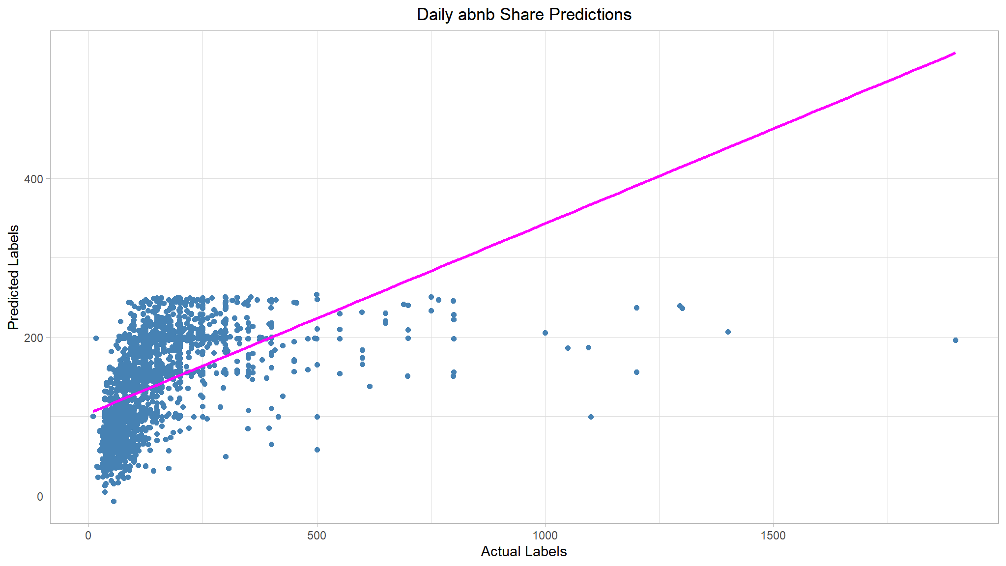

Note

📈There is’nt a definite diagonal trend, and the intersections of the predicted and actual values are generally following not really following the path of the trend line; but there’s a fair amount of difference between the ideal function represented by the line and the results. This variance represents the residuals of the model - in other words, the difference between the label predicted when the model applies the coefficients it learned during training to the validation data, and the actual value of the validation label. These residuals when evaluated from the validation data indicate the expected level of error when the model is used with new data for which the label is unknown.

You can quantify the residuals by calculating a number of commonly used evaluation metrics. We’ll focus on the following three:

Mean Square Error (MSE): The mean of the squared differences between predicted and actual values. This yields a relative metric in which the smaller the value, the better the fit of the model
Root Mean Square Error (RMSE): The square root of the MSE. This yields an absolute metric in the same unit as the label (in this case, numbers of price). The smaller the value, the better the model (in a simplistic sense, it represents the average number of price by which the predictions are wrong!)
Coefficient of Determination (usually known as R-squared or R2): A relative metric in which the higher the value, the better the fit of the model. In essence, this metric represents how much of the variance between predicted and actual label values the model is able to explain.

# Multiple regression metrics
eval_metrics <- metric_set(rmse, rsq)

# Evaluate RMSE, R2 based on the results
eval_metrics(data = results,
             truth = price,
             estimate = predictions) %>% 
  select(-2)
#> # A tibble: 2 × 2
#>   .metric .estimate
#>   <chr>       <dbl>
#> 1 rmse      109.   
#> 2 rsq         0.245

Note

Great job 🙌! So now we’ve quantified the ability of our model to predict the number of price.
the model however is not perfoming very well , we would need the follow of RMSE to be at least as little as possible

Trying out other regression algorithms

The linear regression algorithm we used to train the model has some predictive capability, but there are many kinds of regression algorithm we could try, including:

Linear algorithms: Not just the Linear Regression algorithm we used above (which is technically an Ordinary Least Squares algorithm), but other variants such as Lasso and Ridge.
Tree-based algorithms: Algorithms that build a decision tree to reach a prediction.
Ensemble algorithms: Algorithms that combine the outputs of multiple base algorithms to improve generalizability.

Try Another Linear Algorithm

Let’s try training our regression model by using a Lasso (least absolute shrinkage and selection operator) algorithm. Here we’ll set up one model specification for lasso regression; I picked a value for penalty (sort of randomly) and I set mixture = 1 for lasso (When mixture = 1, it is a pure lasso model).

For convenience, we’ll rewrite the whole code from splitting data to evaluating model performance.

# Split 70% of the data for training and the rest for tesing
set.seed(2056)
abnb_split <- out_new_data %>% 
  initial_split(prop = 0.7, strata = price)

# Extract the data in each split
abnb_train <- training(abnb_split)
abnb_test <- testing(abnb_split)

# Build a lasso model specification
lasso_spec <-
  # Type
  linear_reg(penalty = 1, mixture = 1) %>% 
  # Engine
  set_engine('glmnet') %>% 
  # Mode
  set_mode('regression')

# Train a lasso regression model
lasso_mod <- lasso_spec %>% 
  fit(price ~ ., data = abnb_train)

# Make predictions for test data
results <- abnb_test %>% 
  bind_cols(lasso_mod %>% predict(new_data = abnb_test) %>% 
              rename(predictions = .pred))

# Evaluate the model
lasso_metrics <- eval_metrics(data = results,
                                    truth = price,
                                    estimate = predictions) %>%
  select(-2)


# Plot predicted vs actual
lasso_plt <- results %>% 
  ggplot(mapping = aes(x = price, y = predictions)) +
  geom_point(size = 1.6, color = 'darkorchid') +
  # overlay regression line
  geom_smooth(method = 'lm', color = 'black', se = F) +
  ggtitle("Daily abnb Share Predictions") +
  xlab("Actual Labels") +
  ylab("Predicted Labels") +
  theme(plot.title = element_text(hjust = 0.5))

# Return evaluations
list(lasso_metrics, lasso_plt)
#> [[1]]
#> # A tibble: 2 × 2
#>   .metric .estimate
#>   <chr>       <dbl>
#> 1 rmse      109.   
#> 2 rsq         0.244
#> 
#> [[2]]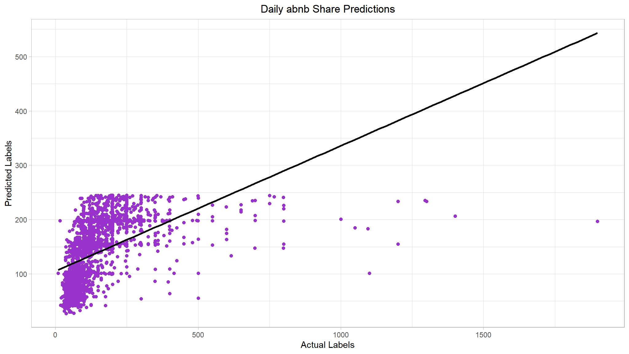

Not much of an improvement. We could improve the performance metrics by estimating the right regularization hyperparameter penalty. This can be figured out by using resampling and tuning the model which we’ll discuss in just a few.

Decision Tree Algorithm

As an alternative to a linear model, there’s a category of algorithms for machine learning that uses a tree-based approach in which the features in the dataset are examined in a series of evaluations, each of which results in a branch in a decision tree based on the feature value. At the end of each series of branches are leaf-nodes with the predicted label value based on the feature values.

The Decision Trees Chapter in Hands-on Machine Learning with R will provide you with a strong foundation in decision trees.

It’s easiest to see how this works with an example. Let’s train a Decision Tree regression model using the abnb rental data. After training the model, the code below will print the model definition and a text representation of the tree it uses to predict label values.

# Build a decision tree specification
tree_spec <- decision_tree() %>% 
  set_engine('rpart') %>% 
  set_mode('regression')

# Train a decision tree model 
tree_mod <- tree_spec %>% 
  fit(price ~ ., data = abnb_train)

# Print model
tree_mod
#> parsnip model object
#> 
#> n= 5403 
#> 
#> node), split, n, deviance, yval
#>       * denotes terminal node
#> 
#>  1) root 5403 72714640 137.39130  
#>    2) room_type=Private Room,Shared room 2543 12780030  80.88871 *
#>    3) room_type=Entire place 2860 44597230 187.63110  
#>      6) neighbourhood_location=Bronx,Brooklyn,Queens,Staten Island 1417 12930030 156.83270 *
#>      7) neighbourhood_location=Manhattan 1443 29003250 217.87460  
#>       14) availability_365< 35.5 709  6860435 184.50490 *
#>       15) availability_365>=35.5 734 20590710 250.10760 *

So now we have a tree-based model; but is it any good? Let’s evaluate it with the test data.

# Make predictions for test data
results <- abnb_test %>% 
  bind_cols(tree_mod %>% predict(new_data = abnb_test) %>% 
              rename(predictions = .pred))

# Evaluate the model
tree_metrics <- eval_metrics(data = results,
                                  truth = price,
                                  estimate = predictions) %>% 
  select(-2)


# Plot predicted vs actual
tree_plt <- results %>% 
  ggplot(mapping = aes(x = price, y = predictions)) +
  geom_point(color = 'tomato') +
  # overlay regression line
  geom_smooth(method = 'lm', color = 'steelblue', se = F) +
  ggtitle("Daily abnb Share Predictions") +
  xlab("Actual Labels") +
  ylab("Predicted Labels") +
  theme(plot.title = element_text(hjust = 0.5))

# Return evaluations
list(tree_metrics, tree_plt)
#> [[1]]
#> # A tibble: 2 × 2
#>   .metric .estimate
#>   <chr>       <dbl>
#> 1 rmse      111.   
#> 2 rsq         0.229
#> 
#> [[2]]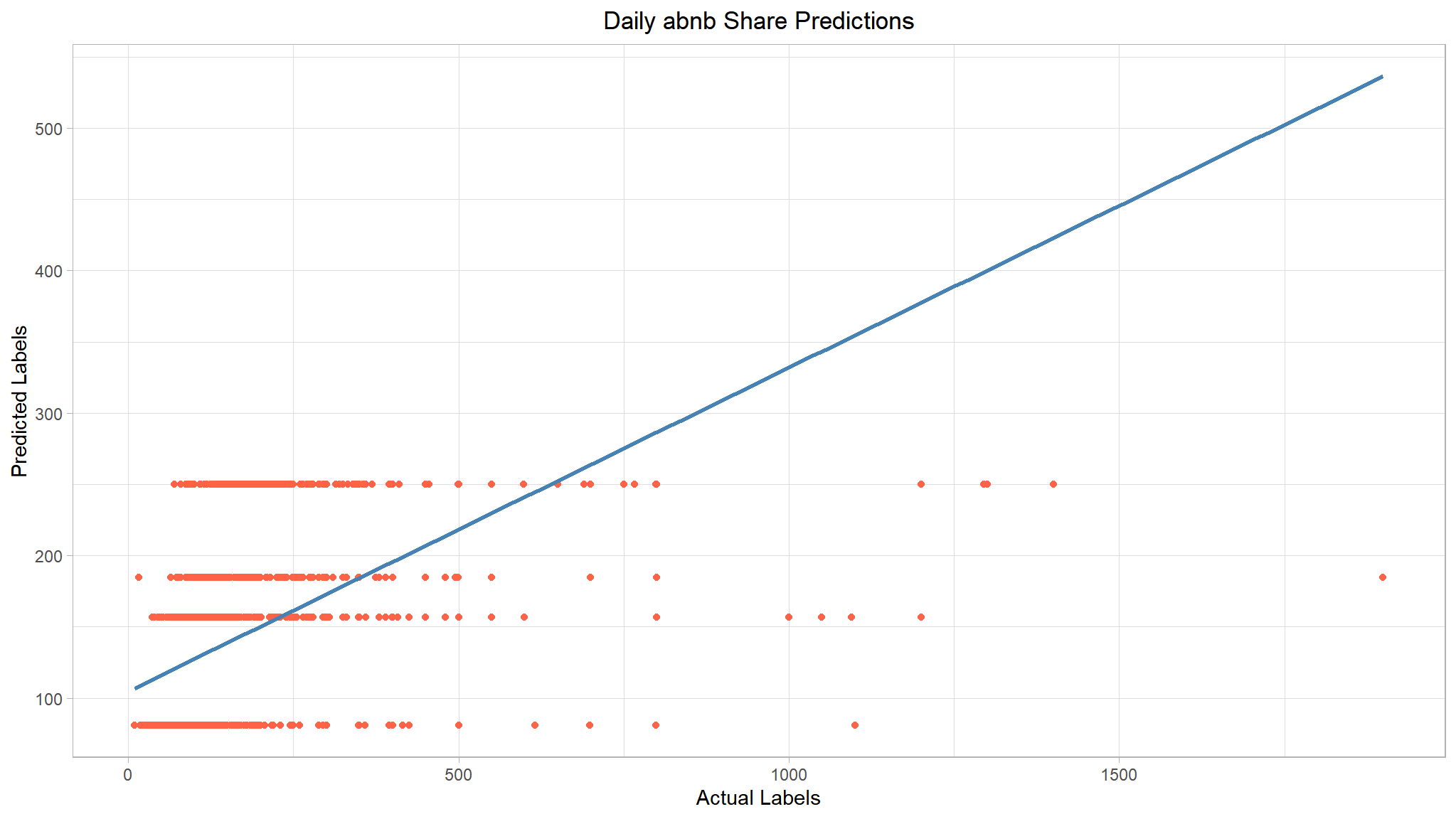

Our decision tree really failed to generalize the data. We can see that it’s predicting constant values for a given range of predictors. We could probably improve this by tuning the model’s hyperparameters.

Ensemble Algorithm

Ensemble algorithms work by combining multiple base estimators to produce an optimal model, either by applying an aggregate function to a collection of base models (sometimes referred to a bagging) or by building a sequence of models that build on one another to improve predictive performance (referred to as boosting).

# Build a random forest model specification
rf_spec <- rand_forest() %>% 
  set_engine('randomForest') %>% 
  set_mode('regression')

# Train a random forest model 
rf_mod <- rf_spec %>% 
  fit(price ~ ., data = abnb_train)


# Print model
rf_mod
#> parsnip model object
#> 
#> 
#> Call:
#>  randomForest(x = maybe_data_frame(x), y = y) 
#>                Type of random forest: regression
#>                      Number of trees: 500
#> No. of variables tried at each split: 2
#> 
#>           Mean of squared residuals: 9774.84
#>                     % Var explained: 27.37

So now we have a random forest model; but is it any good? Let’s evaluate it with the test data.

# Make predictions for test data
results <- abnb_test %>% 
  bind_cols(rf_mod %>% predict(new_data = abnb_test) %>% 
              rename(predictions = .pred))

# Evaluate the model
rf_metrics <- eval_metrics(data = results,
                                  truth = price,
                                  estimate = predictions) %>% 
  select(-2)


# Plot predicted vs actual
rf_plt <- results %>% 
  ggplot(mapping = aes(x = price, y = predictions)) +
  geom_point(color = '#6CBE50FF') +
  # overlay regression line
  geom_smooth(method = 'lm', color = '#2B7FF9FF', se = F) +
  ggtitle("Daily abnb Share Predictions") +
  xlab("Actual Labels") +
  ylab("Predicted Labels") +
  theme(plot.title = element_text(hjust = 0.5))

# Return evaluations
list(rf_metrics, rf_plt)
#> [[1]]
#> # A tibble: 2 × 2
#>   .metric .estimate
#>   <chr>       <dbl>
#> 1 rmse      109.   
#> 2 rsq         0.247
#> 
#> [[2]]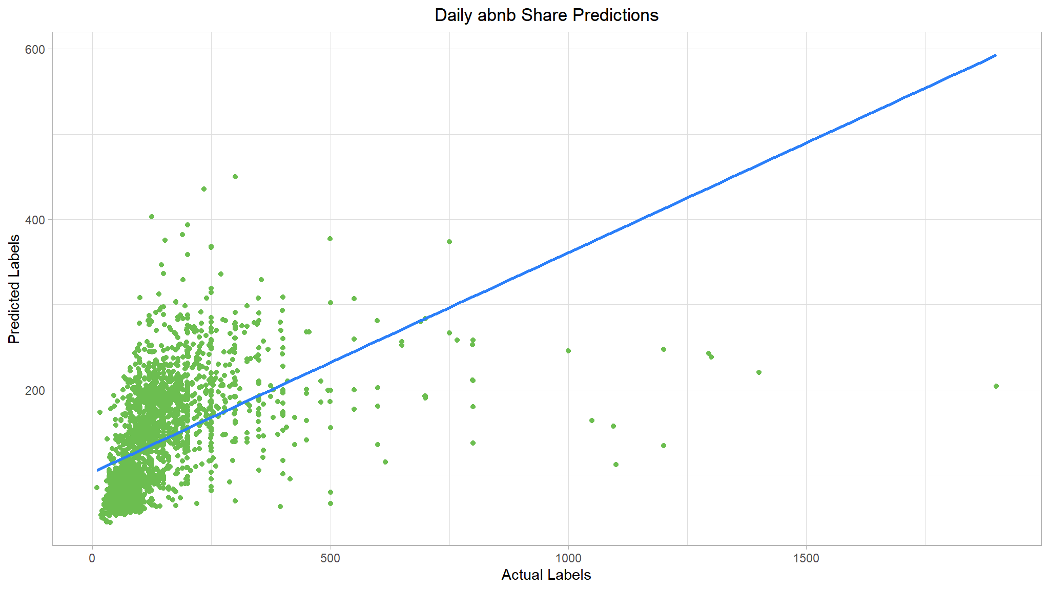

That’s a step in the right direction.Let’s also try a boosting ensemble algorithm. We’ll use a Gradient Boosting estimator, which like a Random Forest algorithm builds multiple trees, but instead of building them all independently and taking the average result, each tree is built on the outputs of the previous one in an attempt to incrementally reduce the loss (error) in the model.

Gradient Boosting Machines

# Build an xgboost model specification
boost_spec <- boost_tree() %>% 
  set_engine('xgboost') %>% 
  set_mode('regression')

# Train an xgboost model 
boost_mod <- boost_spec %>% 
  fit(price ~ ., data = abnb_train)


# Print model
boost_mod
#> parsnip model object
#> 
#> ##### xgb.Booster
#> raw: 69.1 Kb 
#> call:
#>   xgboost::xgb.train(params = list(eta = 0.3, max_depth = 6, gamma = 0, 
#>     colsample_bytree = 1, colsample_bynode = 1, min_child_weight = 1, 
#>     subsample = 1), data = x$data, nrounds = 15, watchlist = x$watchlist, 
#>     verbose = 0, nthread = 1, objective = "reg:squarederror")
#> params (as set within xgb.train):
#>   eta = "0.3", max_depth = "6", gamma = "0", colsample_bytree = "1", colsample_bynode = "1", min_child_weight = "1", subsample = "1", nthread = "1", objective = "reg:squarederror", validate_parameters = "TRUE"
#> xgb.attributes:
#>   niter
#> callbacks:
#>   cb.evaluation.log()
#> # of features: 12 
#> niter: 15
#> nfeatures : 12 
#> evaluation_log:
#>     iter training_rmse
#>        1     141.34842
#>        2     117.66270
#> ---                   
#>       14      74.41446
#>       15      73.87710

From the output, we actually see that Gradient Boosting Machines combine a series of base models, each of which is created sequentially and depends on the previous models, in an attempt to incrementally reduce the error in the model.

So now we have an XGboost model; but is it any good🤷? Again, let’s evaluate it with the test data.

# Make predictions for test data
results <- abnb_test %>% 
  bind_cols(boost_mod %>% predict(new_data = abnb_test) %>% 
              rename(predictions = .pred))

# Evaluate the model
boost_metrics <- eval_metrics(data = results,
                                  truth = price,
                                  estimate = predictions) %>% 
  select(-2)


# Plot predicted vs actual
boost_plt <- results %>% 
  ggplot(mapping = aes(x = price, y = predictions)) +
  geom_point(color = '#4D3161FF') +
  # overlay regression line
  geom_smooth(method = 'lm', color = 'black', se = F) +
  ggtitle("Daily abnb Share Predictions") +
  xlab("Actual Labels") +
  ylab("Predicted Labels") +
  theme(plot.title = element_text(hjust = 0.5))

# Return evaluations
list(boost_metrics, boost_plt)
#> [[1]]
#> # A tibble: 2 × 2
#>   .metric .estimate
#>   <chr>       <dbl>
#> 1 rmse      112.   
#> 2 rsq         0.219
#> 
#> [[2]]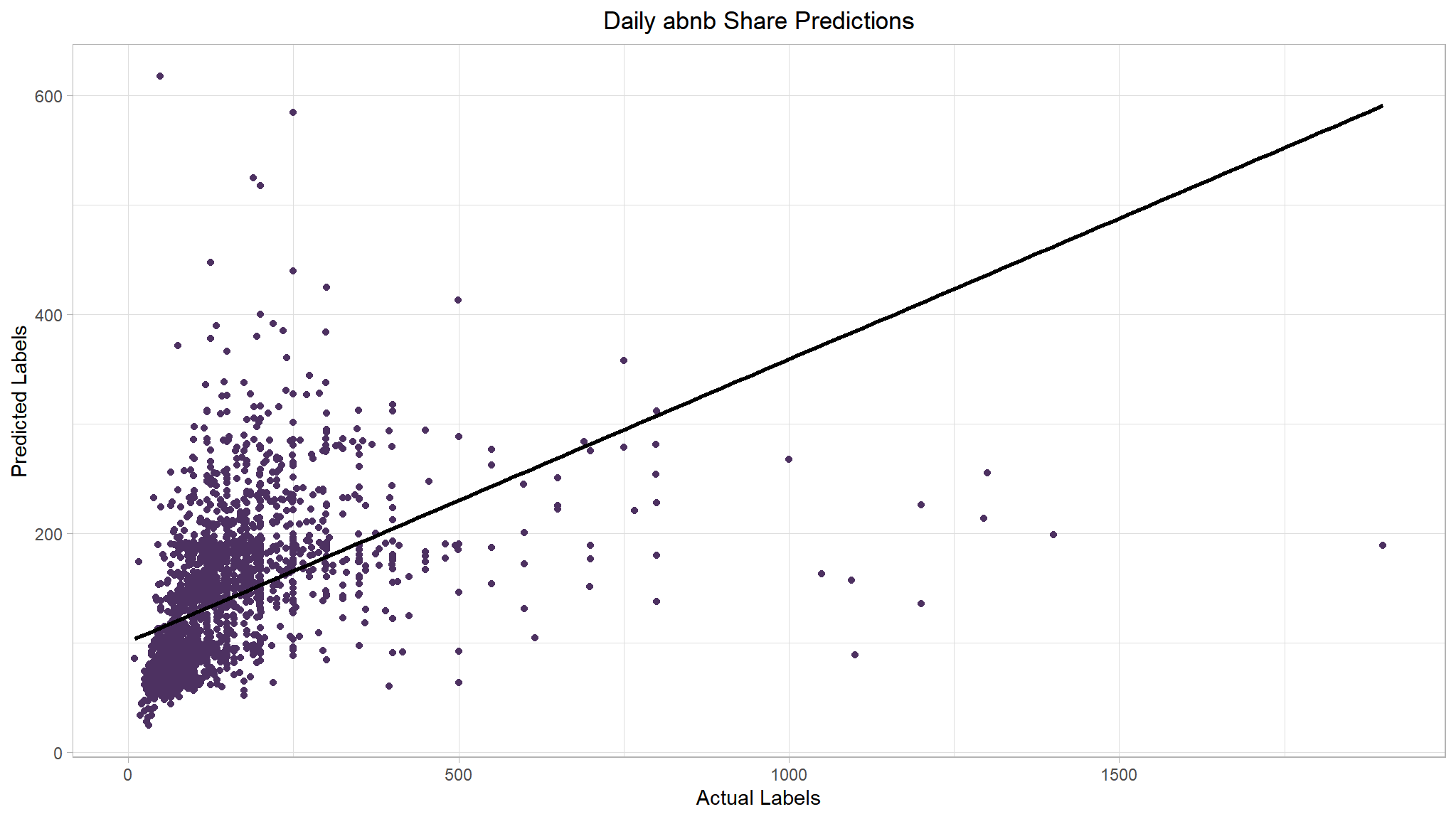

Recipes and Workflows

Preprocess the Data using recipes

There’s a huge range of preprocessing transformations you can perform to get your data ready for modeling, but we’ll limit ourselves to a few common techniques:

Scaling and normalising numeric features

# Specify a recipe
abnb_recipe <- recipe(price ~ ., data = abnb_train) %>% 
  step_normalize(all_numeric_predictors()) %>% 
  step_dummy(all_nominal_predictors()) 

abnb_recipe


# Summary of the recipe
summary(abnb_recipe)
#> # A tibble: 7 × 4
#>   variable               type      role      source  
#>   <chr>                  <list>    <chr>     <chr>   
#> 1 room_type              <chr [3]> predictor original
#> 2 reviews_per_month      <chr [2]> predictor original
#> 3 availability_365       <chr [2]> predictor original
#> 4 rating                 <chr [2]> predictor original
#> 5 number_of_stays        <chr [2]> predictor original
#> 6 neighbourhood_location <chr [3]> predictor original
#> 7 price                  <chr [2]> outcome   original

The call to recipe() with a formula tells the recipe the roles of the variables (e.g., predictor, outcome) using abnb_train data as the reference. This can be seen from the results of summary(abnb_recipe)
step_normalize(all_numeric_predictors()) specifies that all numeric predictors should be normalized.
step_dummy(all_nominal_predictors()) specifies that all predictors that are currently factor or charactor should be converted to a quantitative format (1s/0s).

boost_spec <- boost_tree() %>% 
  set_engine('xgboost') %>% 
  set_mode('regression')

Using a workflow

# Create the workflow
boost_workflow <- workflow() %>% 
  add_recipe(abnb_recipe) %>% 
  add_model(boost_spec)

boost_workflow
#> ══ Workflow ════════════════════════════════════════════════════════════════════
#> Preprocessor: Recipe
#> Model: boost_tree()
#> 
#> ── Preprocessor ────────────────────────────────────────────────────────────────
#> 2 Recipe Steps
#> 
#> • step_normalize()
#> • step_dummy()
#> 
#> ── Model ───────────────────────────────────────────────────────────────────────
#> Boosted Tree Model Specification (regression)
#> 
#> Computational engine: xgboost

# Train the model
boost_workflow <- boost_workflow %>% 
  fit(data = abnb_train)

#boost_workflow

Now, let’s make some predictions on the first 6 observations of our test set.

boost_workflow %>% 
  predict(new_data = abnb_test %>% dplyr::slice(1:6))
#> # A tibble: 6 × 1
#>   .pred
#>   <dbl>
#> 1  81.4
#> 2 220. 
#> 3 220. 
#> 4  72.2
#> 5 131. 
#> 6  91.4

Tune model hyperparameters

Models have parameters with unknown values that must be estimated in order to use the model for predicting. Some model parameters cannot be learned directly from a dataset during model training; these kinds of parameters are called hyperparameters or tuning parameters.

We won’t go into the details of each hyperparameter, but they work together to affect the way the algorithm trains a model. For instance in boosted trees,

min_n forces the tree to discard any node that has a number of observations below your specified minimum.
tuning the value of mtry controls the number of variables that will be used at each split of a decision tree.
tuning tree_depth, on the other hand, helps by stopping our tree from growing after it reaches a certain depth
Learning rate, sets how much a model is adjusted during each training cycle. A high learning rate means a model can be trained faster, but if it’s too high the adjustments can be so large that the model is never ‘finely tuned’ and not optimal

Let us get tuning

# Specify a recipe
abnb_recipe <- recipe(price ~ ., data = abnb_train) %>% 
  step_normalize(all_numeric_predictors()) %>% 
  step_dummy(all_nominal_predictors()) 


# Make a tunable model specification
boost_spec <- boost_tree(trees = 50,
                         tree_depth = tune(),
                         learn_rate = tune()) %>% 
  set_engine('xgboost') %>% 
  set_mode('regression')


# Bundle a recipe and model spec using a workflow
boost_workflow <- workflow() %>% 
  add_recipe(abnb_recipe) %>% 
  add_model(boost_spec)

boost_workflow
#> ══ Workflow ════════════════════════════════════════════════════════════════════
#> Preprocessor: Recipe
#> Model: boost_tree()
#> 
#> ── Preprocessor ────────────────────────────────────────────────────────────────
#> 2 Recipe Steps
#> 
#> • step_normalize()
#> • step_dummy()
#> 
#> ── Model ───────────────────────────────────────────────────────────────────────
#> Boosted Tree Model Specification (regression)
#> 
#> Main Arguments:
#>   trees = 50
#>   tree_depth = tune()
#>   learn_rate = tune()
#> 
#> Computational engine: xgboost

Create a tuning grid.

we’ll need to figure out a set of possible values to try out then choose the best. To do this, we’ll create a grid! To tune our hyperparameters, we need a set of possible values for each parameter to try. In this case study, we’ll work through a regular grid of hyperparameter values.


# Create a grid of tuning parameters
tree_grid <- grid_regular(tree_depth(),
                          # Use default ranges if you are not sure
                          learn_rate(range = c(0.01, 0.3),trans = NULL), levels = 5)

# Display some of the penalty values that will be used for tuning 
tree_grid
#> # A tibble: 25 × 2
#>    tree_depth learn_rate
#>         <int>      <dbl>
#>  1          1     0.01  
#>  2          4     0.01  
#>  3          8     0.01  
#>  4         11     0.01  
#>  5         15     0.01  
#>  6          1     0.0825
#>  7          4     0.0825
#>  8          8     0.0825
#>  9         11     0.0825
#> 10         15     0.0825
#> # ℹ 15 more rows

Let’s sample our data.

hyperparameters cannot be learned directly from the training set. Instead, they are estimated using simulated data sets created from a process called resampling. One resampling approach is cross-validation.

Cross-validation involves taking your training set and randomly dividing it up evenly into V subsets/folds. You then use one of the folds for validation and the rest for training, then you repeat these steps with all the subsets and combine the results, usually by taking the mean. This is just one round of cross-validation. Sometimes practictioners do this more than once, perhaps 5 times.

set.seed(1020)
# 5 fold CV repeated once
abnb_folds <- vfold_cv(data = abnb_train, v = 5, repeats = 1)

abnb_folds
#> #  5-fold cross-validation 
#> # A tibble: 5 × 2
#>   splits              id   
#>   <list>              <chr>
#> 1 <split [4322/1081]> Fold1
#> 2 <split [4322/1081]> Fold2
#> 3 <split [4322/1081]> Fold3
#> 4 <split [4323/1080]> Fold4
#> 5 <split [4323/1080]> Fold5

Time to tune

Now, it’s time to tune the grid to find out which penalty results in the best performance!

doParallel::registerDoParallel()

# Model tuning via grid search
set.seed(2020)
tree_grid <- tune_grid(
  object = boost_workflow,
  resamples = abnb_folds,
  grid = tree_grid
)

Visualize tuning results

Now that we have trained models for many possible penalty parameter, let’s explore the results.

As a first step, we’ll use the function collect_metrics() to extract the performance metrics from the tuning results.

# Extract performance metrics
tree_grid %>% 
  collect_metrics() %>% 
  slice(1:5)
#> # A tibble: 5 × 8
#>   tree_depth learn_rate .metric .estimator    mean     n std_err .config        
#>        <int>      <dbl> <chr>   <chr>        <dbl> <int>   <dbl> <chr>          
#> 1          1       0.01 rmse    standard   137.        5 2.28    Preprocessor1_…
#> 2          1       0.01 rsq     standard     0.193     5 0.00839 Preprocessor1_…
#> 3          4       0.01 rmse    standard   134.        5 2.20    Preprocessor1_…
#> 4          4       0.01 rsq     standard     0.274     5 0.0133  Preprocessor1_…
#> 5          8       0.01 rmse    standard   135.        5 2.06    Preprocessor1_…

Once we have our tuning results, we can both explore them through visualization and then select the best result.

# Visualize the results
tree_grid %>% 
  collect_metrics() %>% 
  mutate(tree_depth = factor(tree_depth)) %>% 
  ggplot(mapping = aes(x = learn_rate, y = mean,
                       color = tree_depth)) +
  geom_line(size = 0.6) +
  geom_point(size = 2) +
  facet_wrap(~ .metric, scales = 'free', nrow = 2)+
  scale_color_viridis_d(option = "plasma", begin = .9, end = 0)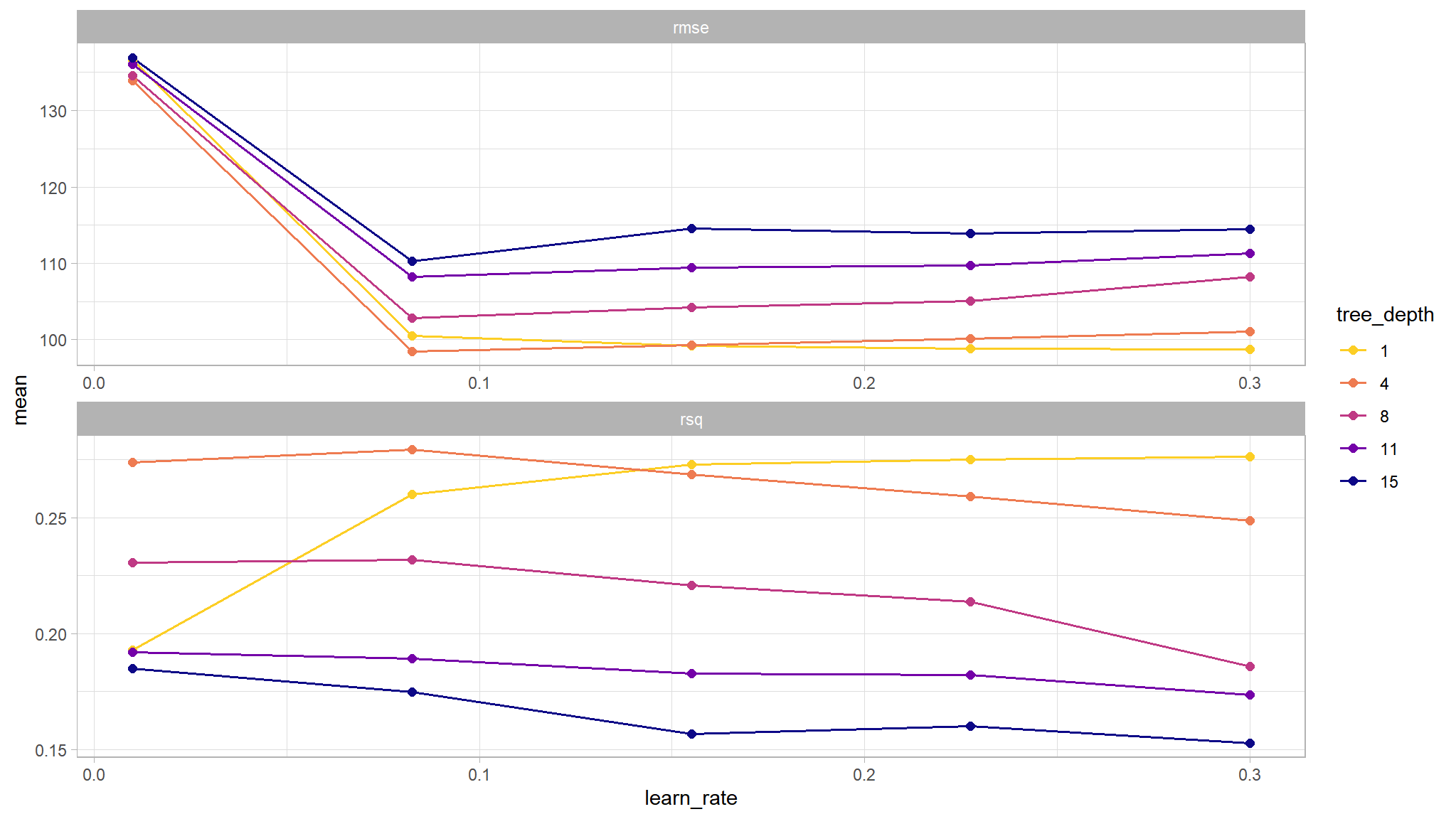

We can see that our “stubbiest” tree, with a depth of 1, is the worst model according to both metrics (rmse, rsq) and across all candidate values of learn_rate. A tree depth of 4 and a learn_rate of 0.1 seems to do the trick! Let’s investigate these tuning parameters further. We can use show_best() to display the top sub-models and their performance estimates.

tree_grid %>% 
  show_best('rmse')
#> # A tibble: 5 × 8
#>   tree_depth learn_rate .metric .estimator  mean     n std_err .config          
#>        <int>      <dbl> <chr>   <chr>      <dbl> <int>   <dbl> <chr>            
#> 1          4     0.0825 rmse    standard    98.5     5    2.32 Preprocessor1_Mo…
#> 2          1     0.3    rmse    standard    98.8     5    2.37 Preprocessor1_Mo…
#> 3          1     0.227  rmse    standard    98.9     5    2.39 Preprocessor1_Mo…
#> 4          1     0.155  rmse    standard    99.2     5    2.42 Preprocessor1_Mo…
#> 5          4     0.155  rmse    standard    99.3     5    2.15 Preprocessor1_Mo…

We can then use select_best() to find the tuning parameter combination with the best performance values.

best_tree <- tree_grid %>% 
  select_best('rmse')

best_tree
#> # A tibble: 1 × 3
#>   tree_depth learn_rate .config              
#>        <int>      <dbl> <chr>                
#> 1          4     0.0825 Preprocessor1_Model07

Finalizing our model

Now that we have the best performance values, we can use tune::finalize_workflow() to update (or “finalize”) our workflow object with the best estimate values for tree_depth and learn_rate.

# Update workflow
final_wf <- boost_workflow %>% 
  finalize_workflow(best_tree)

final_wf
#> ══ Workflow ════════════════════════════════════════════════════════════════════
#> Preprocessor: Recipe
#> Model: boost_tree()
#> 
#> ── Preprocessor ────────────────────────────────────────────────────────────────
#> 2 Recipe Steps
#> 
#> • step_normalize()
#> • step_dummy()
#> 
#> ── Model ───────────────────────────────────────────────────────────────────────
#> Boosted Tree Model Specification (regression)
#> 
#> Main Arguments:
#>   trees = 50
#>   tree_depth = 4
#>   learn_rate = 0.0825
#> 
#> Computational engine: xgboost

Our tuning is done!

The last fit: back to our test set.

Finally, let’s return to our test data and estimate the model performance we expect to see with new data.

# Make a last fit
final_fit <- final_wf %>% 
  last_fit(abnb_split)


# Collect metrics
final_fit %>% 
  collect_metrics()
#> # A tibble: 2 × 4
#>   .metric .estimator .estimate .config             
#>   <chr>   <chr>          <dbl> <chr>               
#> 1 rmse    standard     109.    Preprocessor1_Model1
#> 2 rsq     standard       0.251 Preprocessor1_Model1

there seems to be some improvement in the evaluation metrics compared to using the default values for learn_rate and tree_depth hyperparameters. Now, we leave it to you to explore how tuning the other hyperparameters affects the model performance.

\(\lambda\)	\(Y'\)
2	\(Y^2\)
0.5	\(\sqrt{Y}\)
0	\(ln(Y)\)
-0.5	\(1/\sqrt{Y}\)
-1	\(1/Y\)

library Setup

Simple Regression (Basic Model)

Properties of Least Least Estimators

Residuals

Visualise the relationship graphically

Splitting the data

let us plot a line a best fit (OLS method)

Remember (from High school)

let’s do this in R

let’s solve for intercept

Multiple Linear Regression (Matrix form)

\(\beta_1\)

\(\beta_0\)

Mean Response

Prediction of a new observation

ANOVA

Assumptions

Transformations

Case Study

Top 20 most listed neighborhoods

Data Wrangling

Count of neighborhoods

Mean Price comparison in Each neighborhood

Mean Price comparison in Each room type

Geospatial data

distribution of numeric data

room type by neighhood

correlations

summary statistics

Prepare data for modeling

Building a Regression Model

Evaluate the Trained Model

Compare actual and predictions

Trying out other regression algorithms

Decision Tree Algorithm

Ensemble Algorithm

Gradient Boosting Machines

Recipes and Workflows

Preprocess the Data using recipes

Scaling and normalising numeric features

Using a workflow

Let us get tuning

Create a tuning grid.

Let’s sample our data.

Time to tune

Visualize tuning results

Finalizing our model

The last fit: back to our test set.